Binomial distribution

BINOMIAL DISTRIBUTION

This distribution was discovered by James Bernoulli, though it was published in 1713, eight years after his death.

1. Bernoulli Trial

Each trial has two possible outcomes, generally called success and failure. Such a trial is known as Bernoulli trial.

The sample space for a Bernoulli trial is S = {s, f}

Example:

1. A toss of a single coin [head or tail]

2. The throw of a die [even or odd number]

2. Binomial experiment

An experiment consisting of a repeated number of Bernoulli trials is called Binomial experiment.

A binomial experiment must possess the following properties.

 (i) There must be a fixed number of trials.

 (ii) All trials must have identical probabilities of success (p)

(iii) The trials must be independent of each other.

3. Binomial distribution ■

Consider a set of 'n' independent Bernoullian trials (n being finite), in which the probability p of success in any trial is constant for each trial. Then q = 1- p is the probability of failure in any trial.

A random variable X is said to follow binomial distribution if it assumes only non-negative values and its probability mass function is given by

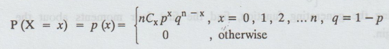
The two independent constants n and p in the distribution are known as the parameters of the distribution. 'n' is also, sometimes known as the degree of the binomial distribution.

Note: Clearly p (x) ≥ 0 for all x and ∑p (x) = (q+p)ⁿ = 1

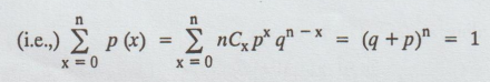
 p (x) is a probability function.

The successive values of probability function are the successive terms in the binomial expansion (q+p)". For this reason the distribution is called binomial distribution.

4. Binomial frequency distribution■

Let us suppose that n trials constitute an experiment. Then if this experiment is repeated N times, the frequency function of the binomial distribution is given by,

f(x) = Np (x) = N nC_xp^x q^{n - x}, x = 0, 1, 2, ... n

The expected frequencies of 0, 1, 2, ... n successes are given by the successive terms of N (q+p)ⁿ.

NOTE: We get the binomial distribution under the following experimental conditions.

(i) Each trial results in two mutually disjoint outcomes, termed as success and failure.

(ii) The number of trials n is finite.

(iii) The trials are independent of each other.

(iv) The probability of success p is constant for each trial.

5. Mode of the Binomial Distribution

Let us find the most probable number of successes in a series of n independent trials with constant probability of success p i.e., we are interested in the number of successes which has the greatest probability. The probability of x successes is given by

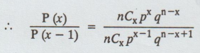
P(x) = nC_xp^x q^n-x

P(x-1)= nC_xp^{x - 1}q^{n – x + 1}

P(X) ≥ or ≤ P(X-1) according as

(n – x + 1)p ≥ or ≤ xq

 (i.e.,) according as (n + 1) p ≥ or ≤ x

og according as x ≥ =  < (n + 1) p

Case 1:

Suppose (n + 1)p is not an integer.

Let m be the integral part of (n + 1) p

But putting x = 1, 2... n we get

P (0) < P (1) < P (2) ... <P (m) > P (m + 1) > P (m + 2) .... > P (n)

Therefore the greatest probability is obtained if the random variable takes the value m, the integral part of (n + 1)p

Case 2:

Suppose (n+1)p is an integer

Let (n + 1) p = m where m is an integer

Proceeding as in case 1 we get

P (0) < P (1) < ... < P (m − 1) = P(m) > P (m + 1) > .... > P (m)

Therefore the greatest probability is obtained when X takes the value of m or (m-1). Hence in this case there are two modes for the binomial distribution.

6. Additive properties of Binomial random variable

If X₁ and X₂ are two independent binomial random variables with parameters (p, n₁) and (p, n₂) then X₁ + X₂ is a binomial RV with parameters (p, n₁ +  n₂).

7. The moment generating function of a binomial distribution about the mean np

On My (t) = (pe_t + q)_n

Differentiating w.r.to 't' and let t = 0, we get

m₁= [n (pe_t + q)^{n - 1}pe^t]_t = 0

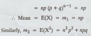
Var (X) = E(X²) – [E(X)]²

= n²p² + npq – n²p²

If X and Y are 2 independent R.Vs having the moment generating function.

M_X (t) = (P₁e^t +q₁)ⁿ¹ and M^Y (t) = (P₂ e^t + q₂)ⁿ²

Then the moment generating function of X + Y is

[ M_{X + Y} (t) = M_X (t). M_Y (t) = (P₁e^t +q₁)ⁿ¹ (P₂ e^t +q₂)ⁿ²

If p₁ = P₂ = p and q₁= q₂ = q, then

M_{X + Y} (t) = (pe^t + q)^{n1 + n2}

8. The first four moments from the moment generating in M_X (pe^t + q)ⁿ¹⁺ⁿ²

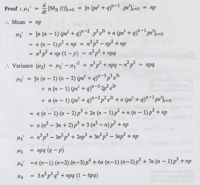
Proof :

Note:

P [exactly 3] = P [equal to 3] = P(X = 3]

P [atmost 3] = P [not more than 3]

 = P [not greater than 3] = P(X ≤ 3]

P [atleast 3] = P [not fewer than 3]

= P [not less than 3] = P[X≥ 3]