Central limit theorem

CENTRAL LIMIT THEOREM

[for independent and identically distributed random variables]

The most widely used model for the distribution of a random variable is a normal distribution. Whenever a random experiment is replicated, the random variable that equals the average result over the replicates tends to have a normal distribution as the number of replicates becomes large. De Moivre presented this fundamental result, known as the central limit theorem, in 1733.

The central limit theorem says that the probability distribution function of the sum of a large number of random variables approaches a gaussian distribution. Although the theorem is known to apply to some cases of statistically dependent random variables, most applications, and the largest body of knowledge are directed towards statistically independent random variables.

It not only provides a simple method for computing approximate probabilities for sums of independent random variables, but it also helps explain the remarkable fact that the empricial frequencies of so many natura populations exhibit bell shaped (that is, normal) curves.

The first version of the central limit theorem was proved by De Moivre around 1733. This was subsequently extended by Laplace (the Newton of France) Laplace also discovered the more general form of the central limit theorem which is given. His proof, however, was not completely rigorous and, in fact, cannot easily be made rigorous. A truly rigorous proof of the central limit theorem was first presented by the Russian mathematician Liapounoff in the period 1901 - 1902.

The application of the central limit theorem to show that measurement errors are approximately normally distributed is regarded as an important contribution to science. Indeed, in the seventeenth and eighteenth centuries the central limit theorem was often called the "law of frequency of errors".

1. Central Limit Theorem: [Lindberg-Levy's form] [A.U A/M 2004, N/D 2010, A/M 2010, N/D 2011] [A.U M/J 2013, N/D 2013]

Statement :

If X₁, X₂, ..., X_n be a sequence of independent identically distributed random variables with E [X_i] = μ and Var [X_i] = σ², i = 1, 2, ..., n and if S_n = X₁ + X₂ + ... + X_n, then under certain general conditions, S_n follows a normal distribution with mean 'n µ' and variance 'n σ² as n → ∞

Proof : Given :

(a) X₁, X₂, ..., X_n be 'n' independent and identically distributed r.v's

(b) E[X₁] = E[X₂] = E[X_n] = µ

(c) Var [X₁] = Var [X₂] = Var [X_n] = σ²

(d) S_n = X₁+ X₂ + ... + X_n

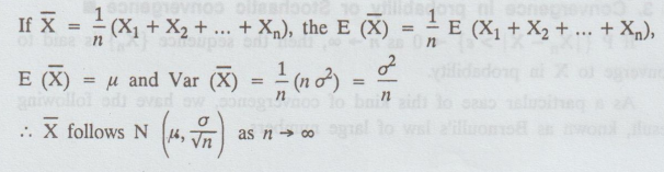
To prove : (1) Mean of S_n = n µ

(2) Var [S_n] = n σ²

(3) S_n must be a normal variate with mean 'n u' and s.d. 'o σ √n'

By using uniqueness property of m.g.f, the variate. Z must be a standard normal variate as n → ∞

Z = S_n – n µ / σ√n

S_n must be a normal variate having (mean = n µ) and (s.d = √σ n)

Thus, as n → ∞, S_n ~ N[n µ, n σ²]

Hence the proof.

Result 1:

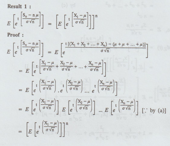
Result 2:

2. Convergence everywhere and almost everywhere

If {X_n} is a sequence of RVs and X is a RV such that it [X_n] = X,

i.e., X_n → X as ∞, then the sequence {X_n} is said to converge to X everywhere.

If P {X_n → X} = 1 as n→ ∞, then the sequence {X_n} is said to converge to X almost everywhere.

3. Convergence in probability or Stochastic convergence

If P { |X_n – X| > ε} → 0 as n → ∞, then the sequence {X_n} is said to converge to X in probability.

As a particular case of this kind of convergence, we have the following result, known as Bernoulli's law of large numbers.

If X represents the number of successes out of 'n' Bernoulli's trials with probability of success P (in each trial), then {X/n} converges in probability to P.

i.e., P ( | X/n – P | > ε } → 0  as n → ∞

4. Convergence in the mean square sense

If E {|X_n - X|²} → 0 as n → ∞ then the sequence {X_n} is said to converge to X in the mean square sense.

5. Convergence in distribution

If Fn (x) and F(x) are the distribution functions of Xn and X respectively such that Fn (x) F(x) as n → ∞ for every point of continuity of F(x), then the sequence {X} is said to converge to X. in distribution.

Note: Closely associated to the concept of convergence in distribution is a remarkable result known as central limit theorem, which is given below without proof.

6. Central limit theorem (Liapounoff's Form)

If X₁, X₂, ... X_n be a sequence of independent RVs with E(X_i) = µ_i and Var (X_i) = σ²_i, i = 1, 2, ... n and if Sn = X1 + X2 + ... + Xn then under certain general conditions, S_n follows a normal distribution with mean

7. Central limit theorem (Lindberg-Levy's form)

[A.U A/M 2019 (R17) PQT]

If X₁, X₂, ... X_n be a sequence of independent identically distributed RV's with E (X_i) = μ and Var (X_i) = σ², I = 1, 2, … n and if S_n =  X₁ + X₂ + ... + X_n, then under certain general conditions, S_n follows a normal distribution with mean nu and variance n σ² as n→ ∞.

8. Corollary

9. Normal area property

The normal variable 'Z' is defined as Z = X – μ / σ

Note that E(Z) = 0; V(Z) = 1. The std. normal distribution is

10. Uses of Central Limit Theorem

(1) It is very useful in statistical surveys for a large sample size. It helps to provide fairly accurate results.

(2) It states that almost all theoretical distributions converge to normal distribution as n→ ∞

(3) It helps to find out the distribution of the sum of a large number of independent random variables.

(4) It also helps explain the remarkable fact that the emprical frequencies of so many natural populations exhibit bell shaped (i.e. normal) curves. [(0)4.8.s olqmaxi

Theorem :

Show that the central limit theorem holds good for a sequence {X_k}, if

P{X_k = ± K^ɑ } = 1/2 XK ^-2α, P{X_k = 0} = 1 − K ^-2α, ɑ < 1/2

Proof: We have to verify that the condition given in the above note is satisfied by the given sequence { X_k}.

 (i.e.,) the necessary condition is satisfied. Therefore CLT holds good for the sequence {X_k}.

TYPE 1: If the average of random variables follows Normal distribution,