Circle Diagram

Circle Diagram.

We had already seen in the previous sections how to calculate the real and reactive power at sending end and at the receiving end mathematically. Now we will see how to represent characteristics of transmission line graphically. By taking either V_S,V_R,I_S or I_R as a reference these characteristics can be plotted. These characteristics are nothing but representing circles. Hence such diagrams are called circle diagram. A circle diagram is drawn with real power P on X-axis and Q on Y axis on complex plane. The circle diagram can be drawn at the sending end as well as at the receiving end.

These diagrams are helpful for determination of active power P, reactive power Q, power angle δ, power factor for given load conditions, voltage conditions and impedance Z of the line.

Receiving End Circle Diagram :

The complex power at the receiving end is given by,

This complex power can be plotted in the complex plane with horizontal and vertical components having the units of powers. This is shown in Fig. 2.15.1.

The real component of (P_R +jQ_R) is,

P_R = |V_R| |I_R| COS θ_R where θ_R is p.f. at the receiving end

The imaginary component of (P_R +jQ_R) is,

Q_R = |V_R| |I_R| sin θ_R

Here θ_R is the phase angle by which I_R lags behind V_R . By convention we will consider that inductive load draws positive reactive power. 

Now if the same phasor diagram shown in Fig. 2.15.1 is redrawn with the origin of the co-ordinates axes shifted, then the resultant figure is shown in Fig. 2.15.2.

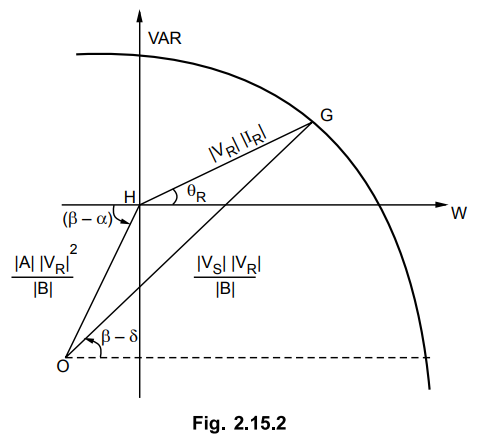
Now we will show that the locus of operating point is a circle with centre at O. For this consider the phasor diagram shown in Fig. 2.15.4. (Refer Fig. 2.15.4 on 2-78).

It can be shown that for constant values of VR and V s and for variable values of IR, the point G moves on a circle with centre O.

In Δ OGH

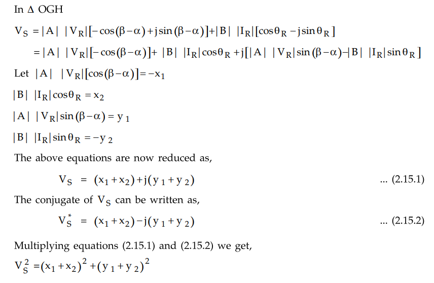
The above equation represents a circle with its centre at O and having co-ordinates (-x₁,-y₁) 

All the phasors shown in Fig. 2.15.3 represent voltage. In order to represent them as volt amperes, multiply each phasor by constant V_R/B which resperents a current phasor because B has dimensions of impedance.

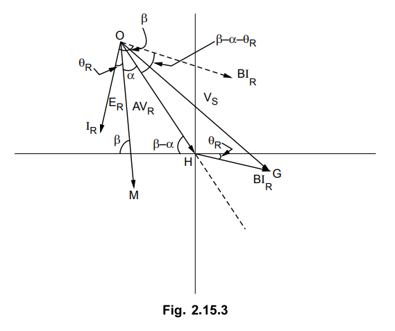
The co-ordinates of the centre of the receiving end circle are given as

The θ_R is the phase angle by which V_R leads I_R. The position of point O is independent of load current I_R and will not change as long as |VR| is constant. Further more if values of V_S and V_R are constant then distance OG remains constant. Now with change in load, the distance between points H and G goes on changing. As the values of V_S andV_R are fixed, distance between points O and G remains same which constrain point G to move on a circle with centre at O and radius as OG. In order to keep point G on the circle it is required that with change in P_R,Q_R should also change.

If values of sending end voltages are changed then for same values |V _R | the position of point O is unchanged but a new circle with different radius is obtained.

With constant receiving end voltage, different circles can be obtained for different values of sending end voltages. The circles so obtained are concentric circles as the location of centre of receiving end power circle is independent of sending end voltage. 

Number of concentric circles can be obtained for a constant receiving end voltage. This is shown in Fig. 2.15.4.

From the Fig. 2.15.4, it can be seen that there is limit to the power that can be transmitted to the receiving end of the line for various magnitudes of sending and receiving end voltages. An increase in power delivered means that point G will move along the circle until the angle β - δ is zero, us so long as δ = β, maximum power is delivered. With further increase in δ, results in less power at receiving end. The equation for maximum power is given by,

As shown in the Fig. 2.15.5 if a vertical line is drawn from x on circle with sending end voltage |VS3 | to the point y on circle with sending end voltage |V _S2| then distance xy represents the amount of negative reactive power that must be drawn by capacitors added in parallel with the load to maintain constant |V _R | when sending end voltage is reduced from |V _S3|  to |V _S2|.

Thus circle diagram helps us to study various aspects of power transmission at sending end and receiving end. From the receiving end power circle diagram, P_R,Q_R and angle δ for any point on the circle can be determined.

For a short transmission line with series impedance per phase as Z ∠ _{θ l.}

For a short line

The circle diagram is as shown in Fig. 2.15.6

1. Procedure to Draw Receiving End Circle Diagram

In this section we will consider the general procedure for drawing circle diagram at receiving end with considerations of various conditions.

Normally in 3 phase system, 3 phase power is specified and the voltage is line to line. The procedure for drawing circle diagram is based on phase quantities.

1) P_R is the receiving end power and V_R is line to line voltage.

P_{R phase} = P_R / 3,    V_{R phase} = V_R / √3

2) Calculate | A |  |V_Rph|² / | B |

3) By checking values of P_Rph and | A |  |V_Rph|² / | B | decide suitable scale.

4) Draw horizontal and vertical axes and fix the centre of the circle whose co-ordinates are given as

Draw line OO₁ as shown in Fig. 2.15.7.

5) From point O₁ draw a load line subtending an angle of θ_R. Reduce P_Rph to scale and cut the horizontal line at point M. Draw the vertical line from this point which will cut the slanted line at L. Thus the operating point L is obtained.

6) Now join OM which is radius of the circle. Convert it by using scale to MVA or kVA

OM × Scale = | V_S | | V_R | / | B |

From above equation |V_S| can be obtained. The phase value of V_S is obtained. Multiply it by √3 to get line to line value for V_S. This part describes the unregulated system where V_S can take any value depending on load condition.

In a regulated system, the receiving end and the sending end voltage is kept same by installing some reactive power injecting device at receiving end.

Under this condition first four steps are repeated. The radius of new circle is |V_S| |V_R| / | B | and with scale draw a circle with same centre.

This arc can intersect ML at any one of three positions of L' as shown in Fig. 2.15.7. i.e. above L, in between L and horizontal or below the horizontal line. If L' is above L, the phase modifier is said to be underexcited. The capacity of the phase modifier in all three cases is L L'. The VAR requirements of load are fixed and are equal to LM.

In underexcited condition, the VARs transmitted over the line are L'M. The transmission line has to transmit VARs required by load as well as supply VARs to phase modifier also which is equal to LL' i.e. phase modifier takes lagging VARs from the system which corresponds to underexcited condition.

When L' lies between L and M, VARs required by load, LL' is supplied by phase modifier and L' M have to be transmitted over the line. The phase modifier is overexcited.

When L' is below horizontal axis, the capacity of phase modifier is LL'. Here the phase modifier supplies VAR requirements of load (LM) as well as sup plies L' M VARs to the transmission line. The phase modifier is overexcited.

The power factor of load is fixed and is given by cos 0 R. If point L' lies above horizontal axis p.f. is lagging and if it lies below horizontal axis it is leading. NP gives the maximum power. 

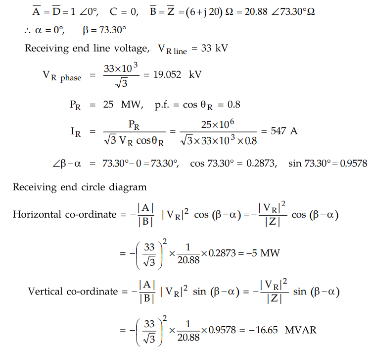
Example 2.15.1 A 3 phase overhead, line has resistance and reactance per phase of 6 Ω and 20 Ω respectively. The load at the receiving end is 25 MW, 33 kV at 0.8 p.f. lagging. Find the voltage at the sending end by drawing receiving end power circle diagram.

AU : Oct.-98, Marks 15

Solution. : As the capacitance of the line is neglected, the line is treated as short transmission line so the ABCD constants will be

Let scales selected be

1 cm = 2 MW on horizontal axis

1 cm = 2 MVAR on vertical axis

So that we have 1 cm - 2 MVA

Steps for drawing the receiving end power circle diagram

1) Locate centre O with co-ordinates as given above. 

2) Draw load line at an angle θ_R = cos^-1 0.8 = 36.8° to the horizontal and cut it at P such that

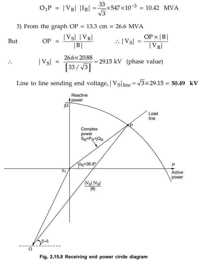
Review Questions

1. Draw and explain how receiving end power circle is found.

2. Explain various steps involved in receiving end power circle diagram, with neat sketches.

3. Write note on receiving end circle diagram.