External Compensation Techniques used in operational amplifiers

External Compensation Techniques

Dec.-07,08,09,10,ll,12,15, May-07,15,17

As mentioned earlier, the compensating network is connected to the system externally to alter the response as per the requirement. There are three such external compensation techniques used in practice.

1) Dominant pole compensation

2) Pole-Zero compensation

3) Feed-forward compensation

1. Dominant Pole Compensation

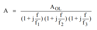
Consider an op-amp with three break frequencies and its loop gain is say A.

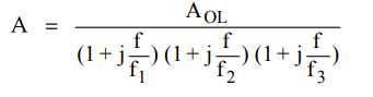
The equation is same as (2.32.1) of section 2.32 and reproduced for the  convenience.

In this loop gain, the dominant pole is introduced by adding a compensating network. Such a network is nothing but a simple R-C network as shown in the Fig. 2.33.1. 

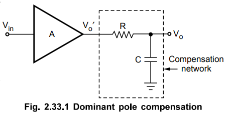
The dominant pole means the pole with magnitude much smaller than the existing poles. And hence the break frequency of the compensating network is the smallest compared to the existing break frequencies.

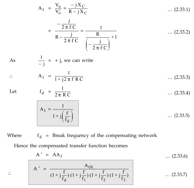
The transfer function of the compensating network can be obtained as :

A1 = Transfer function of compensating network

= Vo / V’o

By the voltage divider rule applied to the network

The values of R and C are selected in such a way that the loop gain drops to 0 dB with a slope of -20 dB/decade and at a frequency where the poles of uncompensated system contributes very small phase shift. This ensures that at ω = ωgc, the phase shift ϕ(f) is greater than -180° and hence positive phase margin. Generally fd is selected so that magnitude plot for A' passes through 0 dB at the pole f1 of A i.e. ωgc = fi- The uncompensated and compensated magnitude plots are shown in the Fig. 2.33.2.

It can be observed from the plot that 3 dB down bandwidth for noncompensated system is BW1 while for compensated it becomes BW2. There is drastic reduction in the bandwidth.

Advantages :

i) As the noise frequency components are outside the smaller bandwidth, the noise immunity of the system improves.

ii) Adjusting value of fd, adequate phase margin and the stability of the system is assured.

Disadvantage :

i) The only disadvantage of the method is that the bandwidth reduces drastically, as mentioned earlier.

2. Pole – Zero Compensation

Consider the same op-amp described by the open loop gain A with three break frequencies as

In this method, the transfer function A is modified by adding a vin pole and a zero with the help of compensating network. The zero added is at higher frequency while a pole is at lower frequency. Such a compensating network is shown in the Fig. 2.33.3. 

The transfer function of the compensating network is say A1.

A1 = Vo / V’o

The values of R1 , R2 and C2 are so selected that the break frequency for the zero matches with the first corner frequency f1 of the uncompensated system. While the pole of the compensating network at fo is selected in such a way that the compensated transfer function A' passes through 0 dB at the second comer frequency f2 of the uncompensated system. The resultant loop gain becomes

A' = AA1 

The first corner frequency is now fo and the gain starts rolling off at -20 dB/decade at f_o. At f = f₁ there is pole-zero cancellation and rolling rate continues as -20 dB/decade. The values of R₁, R₂ and C₂ are selected such that plot passes through 0 dB at f₂ i.e., ω_gc = f₂. The response for f₂ uncompensated and and compensated system is shown in the Fig. 2.33.4

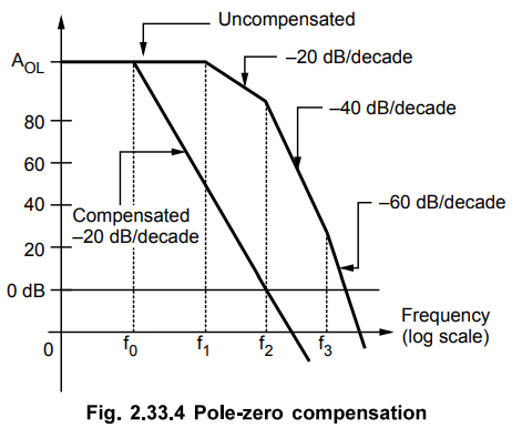
As compared to the dominant pole compensation there is improvement in the bandwidth, equal to f₂ - f₁. This is the additional advantage of pole-zero compensation technique.

The value of compensation capacitor is generally very large. Hence it is not possible to build such capacitor into standard integrated circuits. Generally the connections are brought out from IC to connect the compensation elements externally.

3. Feed-Forward Compensation

In multistage amplifiers it is possible that at gain cross-over frequency d)gc the phase shift may become less than -180° due to individual contributions by the various stages. This is undesirable from the amplifier stability point of view.

Usually there is one stage which is very dominant in providing at least one pole which overrides the effects of other stages hence it acts as bandwidth bottleneck for the over all device. The feed-forward compensation is used to provide a high frequency bypass around such dominant stage to avoid its phase lag. Thus this stage becomes ineffective due to the compensation and the remaining stages provide sufficient phase log in order to obtain a safe value of phase margin.

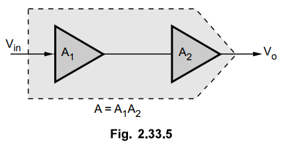
Consider the multistage amplifier with dominant bottleneck stage with response Aj (jf) and all the remaining stages are combined together to get response A2 (jf). The Fig. 2.33.5 shows the two stages while Fig. 2.33.6 shows the individual as well as total frequency response without any compensation used.

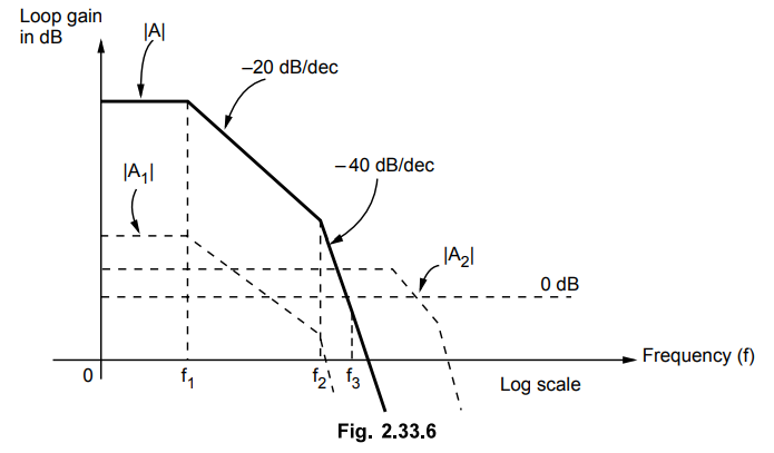
As seen from the frequency response the gain cross-over frequency occurs in the region of roll off 40 dB/dec which indicates instability of the overall system.

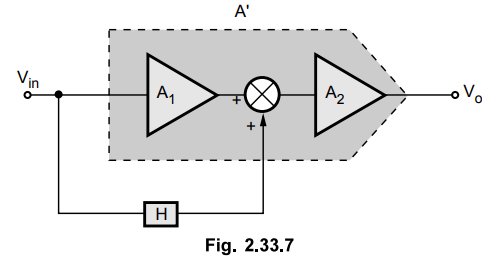
In feed-forward compensation an ordinary high-pass function with transfer function H(jω) is used in the system as shown in the Fig. 2.33.7.

The transfer function of high pass section is,

Now due to this function the overall gain function becomes,

At low frequencies, f → 0 hence H → 0 and hence there is no change in uncompensated response. Thus advantages in low frequency region can be still achieved.

At high frequencies, f → ∞ hence H → l and A → 0 

A' ≈ H(jf) A2 (jf) ≈ A2 (jf) for high frequencies

Thus the system behaviour is controlled by A2 and effect of critical stage A1 is completely eliminated. This gives large bandwidth and gain cross-over frequency occurs now in low roll off region.

The frequency response gets altered as shown in the Fig. 2.33.8.

The disadvantages of this method are :

1. At the time of transition from A to A2, the phase of A may approach to -180° before transition and this may produce excessive ringing effect.

2. If phase lag -180° occurs at transition, signal cancellation results which produces a notch in the compensated response.

In practice feed-forward compensation is provided with a feed-forward capacitor Cc. This is shown for the popular op-amp 101 in the Fig. 2.33.9. The capacitor Cc is connected between the negative terminal (2) and the compensating terminal (1). A small capacitor Cf is needed across Rf to ensure frequency stability.

The expression for the comer frequency of the bypass function is,

fo = 1 / 2πR_ic C_c

where R_ic is the equivalent resistance seen by Cc. This type of compensation gives high slew rate of about 10 V/µs and full-power bandwidth over 200 kHz but it is effective only for inverting type applications.

Review Questions

1. Explain the pole-zero method of frequency compensation.

2. Explain the concept of frequency compensation and discuss any one external compensation technique.

3. Briefly explain the external frequency compensation techniques used in op-amp.