Important Remarks and Observations about Filters

Important Remarks and Observations about Filters

The filter can be represented in the time domain and frequency domain as shown in Fig. 3.5.1 (a) and (b). 

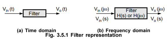
As the filter is frequency selective network, the output V_o(t) contains only some of the frequency components of V_in (t). It is convenient to analyze the filter by representing it in a frequency domain as shown in Fig. 3.5.1 (b). In the frequency domain, the filter is described by the transfer function,

H(s) = V_o (s) / V_in (s) … (3.5.1 a)

or  H(j ω) = V_o (j ω) / V_in (j ω) … (3.5.1 b)

where ω = 2лf and f is the operating frequency. In the steady state, the transfer function can be represented in the polar form as,

The magnitude is generally represented in dB as 20 log |H (jω)|. In the frequency response of various filters discussed above, the magnitude i.e. gain is plotted against the frequency. Thus, the magnitude of the transfer function | H (jω) | = | V_o(j ω) / V_in (j ω) is called gain of the filter. The filters are analy zed and designed considering the magnitude and the phase angle of the transfer function.

An important thing can be observed from the frequency responses discussed above is the behaviour of the gain in the stop band for the various filters. The frequency response either decreases or increases or both in the stop band. The rate at which the gain of the filter changes in the stop band is dependent on the order of the filter. If the filter is first order then gain increases at a rate 20 dB/decade in a stop band of high pass filter, the gain decreases at a rate 20 dB/decade in a stop band of low pass filter and so on. This indicates that there is a change of 20 dB in a gain per decade (10 times) change in the frequency. Such a change in gain is called gain roll off.

Key Point In case of a second order filters, the gain roll off is at the rate of 40 dB/decade and so on.

The various types of filters used in practice which approximately produce the ideal response are : i) Butterworth filters ii) Chebyshev filters iii) Cauer filters.

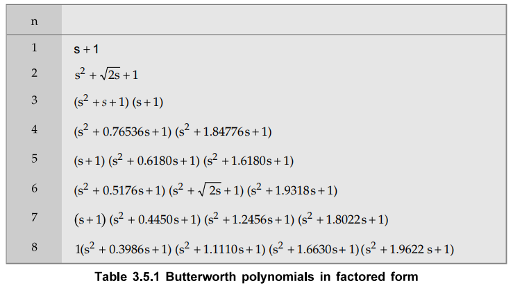
1. Butterworth Approximation

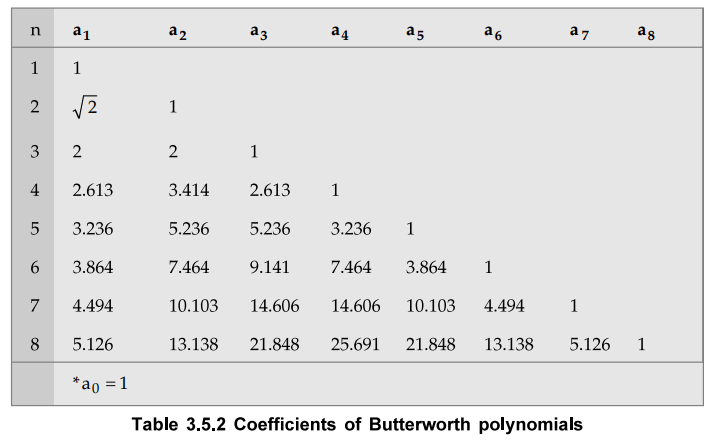
The filter in which denominator polynomial of its transfer function is a Butterworth polynomial is called a Butterworth filter. The Butterworth polynomials of various orders are given in the Tables 3.5.1 and 3.5.2.

The coefficients of Butterworth polynomials are as given in the Table 3.5.2.

Some important observations of Butterworth polynomials expressed in factored form as given in the Table 3.5.2 are as follows : 

1. Coefficient of the highest power of s is always 1 for any order of filter.

2. Lowest order term i.e. constant term is always 1 for any order of filter.

3. For all odd ordered filters, one of the factors is always (s + 1) while the remaining factors are quadratic in nature.

4. For all even ordered filters, all factors are quadratic in nature.

5. All the poles of Butterworth polynomial are located in left half of s-plane on a circle with radius equal to one and centre at origin.

Review Question

1. Write a note on Butterworth approximation.