Instrumentation Amplifiers using Op-amp

Instrumentation Amplifiers

May-03,05,08,11,13,15,16,17, Dec.-03,04,06,08,09,10,11

Many industrial systems, consumer systems and process control systems require a precise measurement of the physical quantities like temperature, pressure, humidity, weight etc. A sugar factory requires a measurement of flow, level and temperature of juice. The plastic furnaces require precise measurement of the temperature. The dairy plant requires a precise measurement of temperature and the humidity. Such measurements help the industries to have the production of quality products.

The measurement of the physical quantities is generally carried out with the help of a device called as transducer. A transducer is a device which converts one form of energy into another. For example a thermocouple converts the heat energy into an electrical energy, microphone converts the sound energy into an electrical energy, strain gauge converts pressure, force like mechanical energy into an electrical energy. Such a proportional electrical signal output from a transducer can be used further to control or operate the other parts of the system or can be used to get the display or recording of the measured physical quantity.

But most of the transducer outputs are generally of very low level signals. Such a low level signals are not sufficient to drive the next stage of the system. One more difficulty in the practical systems is that the transducer used may be mounted on pieces of equipment or structures which are remote from the control location. Long connecting wires or cables are required in such a case, to get the transducer output to the control room. Due to this, the signal which itself is low level, gets subjected to the noise and atmospheric interference. Such a signal may be as low as few mV or even pV.

Hence before the next stage, it is necessary to amplify the level of such signal, rejecting the noise and the interference. Hence general single ended amplifier like high gain emitter amplifier is not suitable to amplify such signals. For rejection of noise, such amplifiers must have high common mode rejection ratio. Hence a special amplifier is used to amplify such signals.

The special amplifier which is used for such a low level amplification with high CMRR, high input impedance to avoid loading, low power consumption and some other features is called an instrumentation amplifier. Such special featured instrumentation amplifiers have become an integral part of modem testing and measurement instrumentation.

The instrumentation amplifier is also called data amplifier and is basically a difference amplifier. The expression for its voltage gain is generally of the form,

A = V_o / V₂ – V₁  …. (3.1.1)

where          V_o = Output of the amplifier 

V₂ – V₁  = Differential input which is to be amplified

Let us list down the requirements of an instrumentation amplifier.

1. Requirements of a Good Instrumentation Amplifier

As mentioned above, the instrumentation amplifiers are used to amplify the low level differential signals very precisely, in presence of the large common mode noise and interference signals. Hence a good instrumentation amplifier has to meet the following specifications :

1) Finite, accurate and stable gain : As very low level signals are required to be amplified by the instrumentation amplifiers, high and finite gain is the basic requirement. It is usually in the range of 1 to 1000. The gain has to be accurate and closed loop gain must be stable in nature.

2) Easier gain adjustment : Not only finite and stable gain is required but a variable gain over the prescribed range is also required. The gain adjustment must be easier and precise. Generally such gain adjustment is done continuously using a potentiometer or is done digitally with the help of switches, which are JFET or MOSFET switches.

3) High input impedance : To avoid the loading of input sources, input impedance of the instrumentation amplifier must be very high (ideally infinite). The differential mode input impedance Z_id is the equivalent impedance between the two input terminals. The common mode input impedance Z_ic is the equivalent impedance between each input terminal and ground.

4) Low output impedance : Extremely low output impedance (ideally zero) to avoid the loading on the immediate stage.

5) High CMRR : The output of transducer, when transmitted with long transmission lines has presence of large common mode noise voltages. The instrumentation amplifier must amplify only the differential input, completely rejecting the common mode input component. Thus it must have ideally infinite CMRR.

6) Low power consumption : The power consumption of an instrumentation amplifier should be as low as possible.

7) Low thermal and time drifts : The parameters of the instrumentation amplifier, should not drift with temperature or time.

8) High slew rate : The slew rate of the instrumentation amplifier must be as high as possible to provide maximum undistorted output voltage swing.

9) The amplifier must have differential input so that it can be amplified.

Let us see the various circuits which can be used as the instrumentation amplifier and their advantages and disadvantages. 

2. Three Op-amp Instrumentation Amplifier

Another commonly used instrumentation amplifier circuit is one using three op-amps. This circuit provides high input resistance for accurate measurement of signals from transducers. In this circuit, a non-inverting amplifier is added to each of the basic difference amplifier inputs. The circuit is shown in the Fig. 3.1.1.

The op-amps A1 and A 2 are the non-inverting amplifiers forming the input or first stage of the instrumentation amplifier. The op-amp A₃ is the normal difference amplifier forming an output stage of the amplifier.

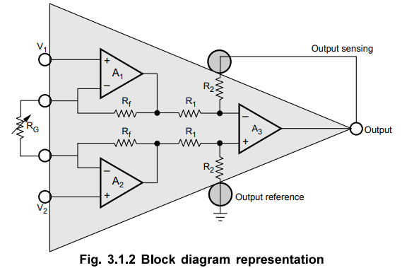
The block diagram representation of the three op-amp instrumentation amplifier is shown in the Fig. 3.1.2.

a. Analysis of Three Op-amp Instrumentation Amplifier

It can be seen that the output state is a standard basic difference amplifier. So if the output of the op-amp A₁ is V_ol and the output of the op-amp A₂ is V_o2, we can write,

V_o = R₂ / R₁ (V_o2 – V_o1) …. (3.1.1)

Let us find out the expression for V_o2 and V_o1 interms of V₁, V₂, R_f1 and R_f2 and R_G.

Consider the first stage as shown in the Fig. 3.1.3.

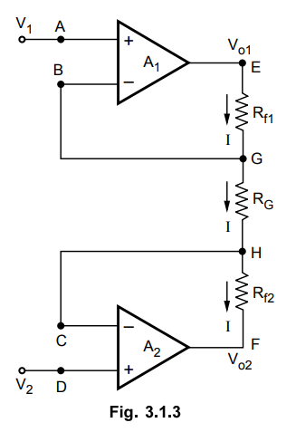
The node A potential of op-amp A₁ is V₁. From the realistic assumption, the potential of node B is also V₁ And hence potential of G is also V₁

The node D potential of op-amp A₂ is V₂. From the realistic assumption, the potential of node C is also V₂. And hence potential of H is also V₂.

The input current of op-amp A₁ and A₂ both are zero. Hence current I remains same through R_fl R_G and R_f2

Applying Ohm's law between the nodes E and F we get,

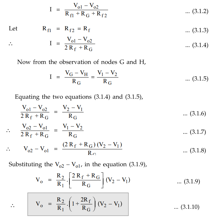
This is the overall gain of the circuit.

 b. Advantages

Following are the advantages of three op-amp instrumentation amplifier circuit :

i) With the help of variable resistance RG, the gain can be easily varied, without disturbing the symmetry of the circuit.

ii) Gain depends on external resistances and hence can be adjusted accurately and made stable by selecting high quality resistances.

iii) The input impedance depends on the input impedance of non-inverting amplifiers which is extremely high.

iv) The output impedance is the output impedance of the op-amp A 3 which is very very low. This is as required by any instrumentation amplifier.

v) The CMRR of the op-amp A 3 is very high and most of the common mode signal will be rejected.

vi) By trimming one of the resistances of the output stage, CMRR can be made extremely high, as required by a good instrumentation amplifier.

Thus the circuit satisfies all the requirements of a good instrumentation amplifier and hence very commonly used in practical applications.

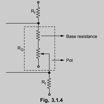
Key Point The resistance RG is generally implemented as the series combination of the suitable base resistance and the pot. This is shown in the Fig 3.1.4.

3. Applications of Instrumentation Amplifier

As mentioned earlier, the instrumentation amplifier along with the transducer bridge can be used in many practical applications. Let us study some of such practical applications. The general form of such systems can be called as 'data acquisition system' and can be represented in the block diagram form as shown in the Fig. 3.1.5.

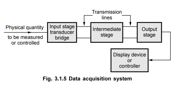
The input stage is a transducer bridge which converts physical quantity to be measured into an electrical signal. The signal is then carried out to an instrumentation amplifier, with the help of transmission lines. The output stage consists of display device, controller or some type of signal conditioning circuit such as ADC etc.

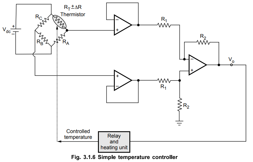
a. Temperature Controller

A simple temperature control circuit can be constructed using thermistor in the transducer bridge. The bridge is set balanced for a particular reference temperature. For any change in this temperature, the instrumentation amplifier produces the output voltage. Now this voltage can be used to drive the relays which intum controls the ON-OFF of the heating unit, to control the temperature.

The system is shown in the Fig. 3.1.6.

b. Temperature Indicator

The circuit shown above in the Fig. 3.1.6 can be used as a temperature indicator. As explained earlier, bridge is kept balanced at some reference temperature when Vo = 0 V. The meter connected at the output is calibrated to reference temperature, corresponding to this reference condition. As temperature changes, amplifier output also changes. The meter can be calibrated to indicate the desired temperature range by selecting the appropriate gain of the amplifier.

c. Light Intensity Meter

The same circuit, replacing thermistor with a photocell can be used as a simple light intensity meter. The bridge is made balanced for the darkness condition. When light falls on the photocell its resistance changes and produces imbalanced bridge condition. This produces the output, which intum produces the meter deflection. The meter can be calibrated in terms of lux to measure the light intensity. Such a light intensity meter is very accurate and stable.

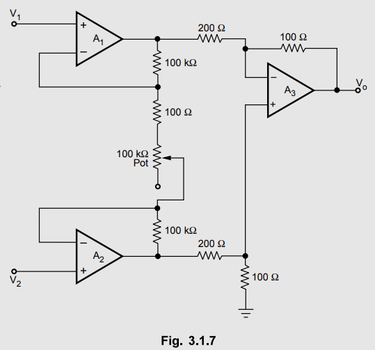
Example 3.1.1 The circuit shown in the Fig. 3.1.7 is an instrumentation amplifier . Determine the range over which its gain can be varied if potentiometer is varied over its entire range.

Solution : The gain of the instrumentation amplifier is given by,

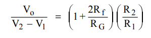
In the circuit given,

R₂ = 100 Ω, R₁ = 200 Ω, R_f = 100 k Ω

And R_G is the series combination of 100 Ω and potentiometer of 100 k Ω. Let potentiometer resistance is 0 Ω at start,

Hence, R_G = 100 + 0 = 100 Ω

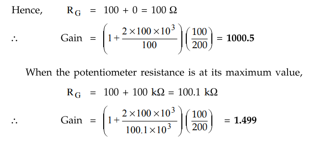
For all practical purposes, the gain can be varied from 1.5 to 1000.5.

Example 3.1.2 For the instrumentation amplifier shown in the Fig. 3.1.8, determine the value of RG if the gain required is 1000.

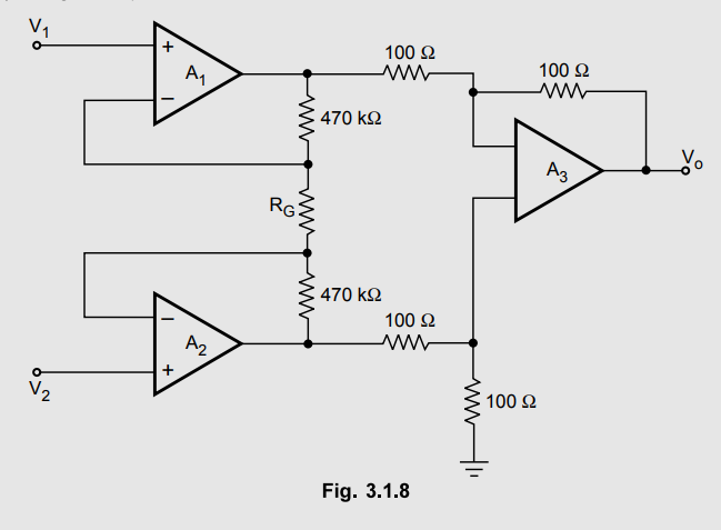
Solution : The values of various resistances are

R₁ = 100 k Ω, R₂ = 100k Ω, R_f = 470 k Ω

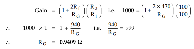
The RG is to be selected for gain of 1000.

Review Questions

1. Draw the instrumentation amplifier using 3 op-amps and derive the expression for the overall gain. Illustrate the features and applications in which this is used. Name any two commonly available instrumentation amplifiers.

May-08, 11, 13, 16, 17, Dec.-06, 08, 10, Marks 16

2. Mention the advantages of three amplifier configuration of an instrumentation amplifiers.

Dec.-06, Marks 6

3. Explain the working of instrumation amplifier.

May-15, Marks 8

4. What are the requirements of good instrumentation amplifier ?