Probability and complex function: Unit II: Two dimensional random variables
Joint distributions - marginal and conditional distributions
Two dimensional random variables
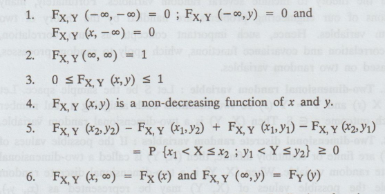
The probabilities of the two events A = {X ≤ x} and B = {Y ≤ y} defined as functions of x and y, respectively, are called probability distribution. functions.
Joint distributions - marginal and conditional distributions.
1. Joint probability distribution
The
probabilities of the two events A = {X ≤ x} and B = {Y ≤ y} defined as
functions of x and y, respectively, are called probability distribution.
functions.
Fx
(x) = P(X ≤ x);
Fy
(y) = P(Y ≤ y)
Note:
We introduce a new concept to include the probability of the joint event {X ≤x,
Y ≤y}.
2. Joint probability distribution of two random variables X and Y
We
define the probability of the joint event {X ≤x, Y ≤y}, which is a function of
the numbers x and y, by a joint probability distribution function and denote it
by the symbol Fx, y (x, y). Hence
Fx,
y (x,y) = p {X ≤ x, Y ≤ y}
Note:
Subscripts are used to indicate the random variables in the bivariate
probability distribution. Just as the probability mass function of a single
random variable X is assumed to be zero at all values outside the range of X,
so the joint probability mass function of X and Y is assumed to be zero at
values for which a probability is not specified.
3. Properties of the joint distribution
A
joint distribution function for two random variables X and Y h several
properties.
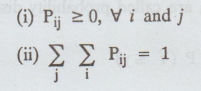
4. Joint probability function of the discrete random variables X and Y
If
(X, Y) is a two-dimensional discrete random variable such that f(xi,
yj) = P(X = xi, Y = yj) = Pij is called
the joint probability function or joint probability mass function of (X, Y)
provided the following conditions are satisfied.
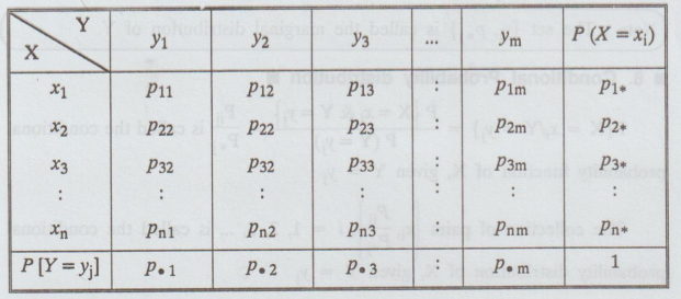
The
set of triples {xi, yj, Pij), i = 1, 2, ... n, j = 1, 2, ... m is called the
joint probability distribution of (X, Y). It can be represented in the form of
table as given below.
5. Marginal probability distribution
If
more than one random variable is defined in a random experiment, it is
important to distinguish between the joint probability distribution of X and Y
and the probability distribution of each variable individually. The individual
probability distribution of a random variable is referred to as its marginal
probability distribution.
In
general, the marginal probability distribution of X can be determined from the
joint probability distribution of X and other random variables.
6. Marginal probability mass function of X
If
the joint probability distribution of two random variables X and Y is given,
then the marginal probability function of X is given by
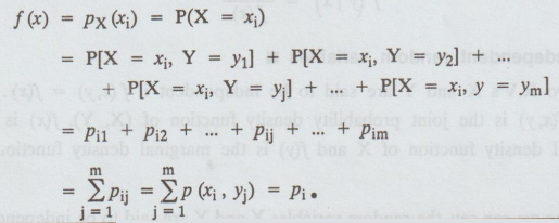
Note:
The set {xi, Pi.} is called the marginal distribution of
X.
7. Marginal Probability mass function of Y
If
the joint probability distribution of two random variables X and Y is given,
then the marginal probability function of Y is given by
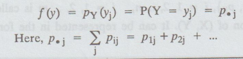
Note:
The set {yi, P.j} is called the marginal distribution of Y.
8. Conditional Probability distribution
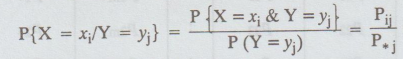 is called the conditional probability function of X, given Y = yj
The
collection of pairs {xi, pij/pi} i = 1, 2, 3, ... is
called the conditional probability distribution of X, given Y = yj
Similarly,
the collection of pairs, {yi, pij/pi} , j = 1, 2, 3, ...
is called the conditional probability distribution of Y given X = xi.
let
(X, Y) be the two dimensional continuous R.V. The conditional probability
density function of X given Y is denoted by f (x | y) and is defined as,
f(x
| y) = f(x, y) / f (y)
Similarly,
the conditional probability density function of Y given X is denoted by f ( y |
x) and is defined as,
f(y
| x) = f(x, y) / f(x)
9. Independent random variables
Two
R.V's X and Y are said to be independent if f (x, y) = f(x).flv) where f(x,y)
is the joint probability density function of (X, Y), f(x) is the marginal
density function of X and f(y) is the marginal density function of Y.
Also
we can say, the random variables X and Y are said to be independent R.V's if
Pij
= Pi* × P*j
where
Pij is the joint probability function of (X, Y), P i* is the
marginal probability function of X and P*j is the marginal probability function of Y.
10. Joint probability density function
If
(X, Y) is a two-dimensional continuous R.V such that
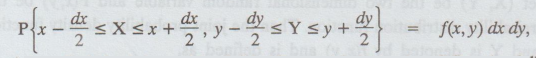
then
f(x, y) is called the joint p.d.f. of (X, Y), provided f(x, y) satisfies the
following conditions.
(i)
f(x, y) ≥ 0, ∀
(x, y) ∈ R, where 'R' is the
range space.
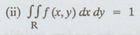
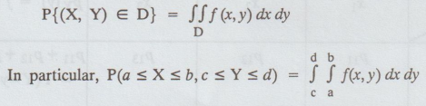
Moreover,
if D is a subspace of the range space R,
P{(X,
Y) E D} is defined as,
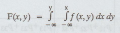
11. Cumulative distribution function
If
(X, Y) is a two-dimensional continuous random variable, then F(x, y) = P(X ≤ x
and Y ≤ y) is called the cdf of (X, Y) and is defined as,
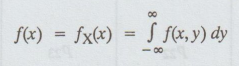
12. Marginal density function
If
(X, Y) is a two-dimensional continuous random variable, then
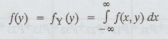
Let
(X, Y) be the two dimensional random variable. Then, the marginal probability
density function of X is denoted by f(x) and is defined as,
Similarly,
the marginal probability density function of Y is denoted by f(y) and is defined
as,
13. Joint probability density function
Let
(X, Y) be the two dimensional random variable and F(x, y) be the joint
probability distribution function. Then the joint probability density function
of X and Y is denoted by f(x, y) and is defined as,
f(x,
y) = ∂2F(x,y) / ∂x ∂y
14. Table I.
To
calculate marginal distributions when the random variable X takes horizontal
values and Y takes vertical values.

15. Table - II
To
calculate marginal distributions when the random variable X takes vertically
and Y takes horizontally.

Probability and complex function: Unit II: Two dimensional random variables : Tag: : Two dimensional random variables - Joint distributions - marginal and conditional distributions
Related Topics
Related Subjects
Probability and complex function
MA3303 3rd Semester EEE Dept | 2021 Regulation | 3rd Semester EEE Dept 2021 Regulation