Latin Square Design

LATIN SQUARE DESIGN

 

1. Introduction :

The term Latin square takes its name from a figure of mathematical puzzle that was studied many years before, use as a plan of experiment.

Latin squares are very extensively used in agricultural trials in order to eliminate fertility trends in two directions, simultaneously. The data are classified according to the different criteria, (i.e.,) according to columns, rows and varieties and are arranged in a square known as Latin Square.

Latin square is one way of reducing the sample size. Suppose, it is desired to study the results of three different types of teaching methods on students. Suppose, the effect on students is also affected by their age bracket and by their aptitude. Our interest is to study the results of the three teaching methods by blocking the effects of age and aptitude. aloval ponsortingia

Now, only nine blocks is to be studied in relation to 3 teaching methods, so in the complete design as many as 27 subjects will have to be studied.

Latin square design is very popular in agricultural research where it is not possible to have a large number of subjects.

Latin squares have an equal number of rows and columns. One blocking factor is represented in the columns of the other in rows. The factor of interest or treatment is within each column and row generally represented by alphabets. Thus, if three teaching methods are to be studied they would be represented by A, B and C. These alphabets are so arranged that each comes only once in a row and only once in a column.

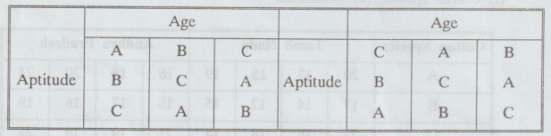
Thus, if three teaching methods A, B and C are to be studied by blocking two factors age and aptitude the latin square would assume the following shape.

 

2. Merits and Demerits of Latin Square Design

Merits

1. Latin Square design controls variability in two directions of the experimental material.

2. The analysis of the design is simple and straight forward and is a three way classification of analysis of variance.

Demerits

1. The process of randomization is not as simple as in RBD.

2. The number of treatments should be equal to the number of rows and boliz number of columns.

3. The experimental area should be in the form of a square.

4. It is suitable only in the case of smaller number of treatments (preferably less than 10).

5. A 2 × 2 Latin Square is not possible.

 

3. Assumption in the Analysis of Latin Square

The Latin Square model assumes that interactions between treatments and row and column groupings are non-existent. Since, each treatment occurs only once in each row or column, if interactions are present, it is possible for them to cause an apparently significant difference between treatments. This is one of the reasons why it is important to choose rows and columns of a particular Latin Square in a random way. Interactions present, can be viewed as random elements that are part of the treatment. They blow up the error variance and make the test less efficient but their randomization still allows for a valid theoretical test.

 

4. Steps in Constructing Latin Square

The construction of Latin Square involves the following steps:

1. Compute the correction factor by squaring the grand total and dividing it by the number of observations.

2. Compute the total sum of squares by adding the squares of the individual observations and subtracting the correction factor.

3. Compute the row sum of squares by adding the squares of the row sums, dividing by the number of items in a row, and subtracting the correction factor.

4. Compute the column sum of squares by adding the squares of the column sums, dividing by the number of items in a column, and subtracting the correction factor.

5. Compute the 'treatment' sum of squares by summing the squares of the treatment sums dividing by the number of treatments, and subtracting the correction factor.

6. Compute the remainder sum of squares by subtracting the sum of 3, 4, and 5 from 2.

7. Enter these sums of squares in an analysis of variance table and compute the various mean squares.

 

5. Working Rule

The analysis is done in a way similar to two-way classification. The different sums of squares are obtained as follows :

Step 1: Find N.

Step 2: Find T.

Step 3: Find T² / N.

Step 4: Find TSS

Step 5: Find SSC

Step 6: Find SSR

Step 7: Find SSK

Step 8: Find SSE

Step 9: ANOVA table

Step 10: Conclusion

 

6. Preparation of ANOVA table

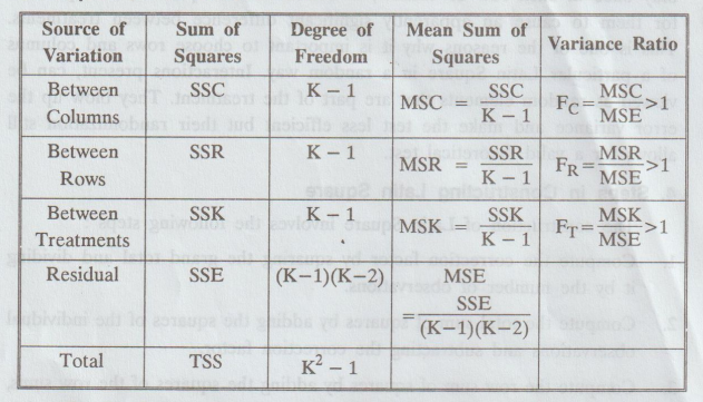
The F-ratios FC, FR, FT are calculated in a such way that they are each greater than one.

For example, if MSC / MSE  < 1, then take Fc = MSE / MSC

 

Example 2.4.1

The following is a Latin square of a design, when 4 varieties of seeds are being tested. Set up the analysis of variance table and state your conclusion. You may carry out suitable change of origin and scale.

Solution: Subtract 100 and then divided by 5, we get

H₀ : There is no significant difference between column means, row means and treatments.

H₁ : There is significant difference between column means or the row means or treatments.

Step 10 Conclusion :

(i) Cal Fe <  Table Fe, i.e., 7.52 < 8.94. So, we accept Ho for this case.

i.e., there is no significant difference between columns.

(ii) Cal FR > Table FR, i.e., 14.93 > 8.94. So, we reject Ho for this case.

i.e., there are significant differences in rows.

(iii) Cal FT< Table FT, i.e., 1.36<8.94. So, we accept Ho for this case.

i.e., there is no significant difference between treatments.

 

Example 2.4.2

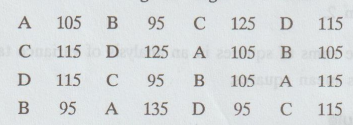
A variable trial was conducted on wheat with 4 varieties in a Latin Square Design. The plan of the experiment and the per plot yield are given below:

Analyse data and interpret the result. [A.U M/J 2012]

[A.U N/D 2016 R-13] [A.U A/M 2017 R-13] [A.U N/D 2019 R-13]

Solution: Subtract 20 from all the items.

H₀ : There is no significant difference between rows, columns and treatments.

H₁ : There is significant difference between rows or columns or treatments.

Step 10 Conclusion :

(i) Cal Fe < Table Fe, i.e., 1.43 < 4.76. So, we accept Ho for this case.

i.e., there is no significant difference between columns.

(ii) Cal FR > Table FR, i.e., 8.86 > 4.76. So, we reject Ho for this case.

i.e., there are significant differences in rows.

(iii) Cal FT > Table Fr, i.e., 9.24>4.76. So, we reject Ho for this case.

 i.e., there are significant difference in treatments.

 

Example 2.4.3

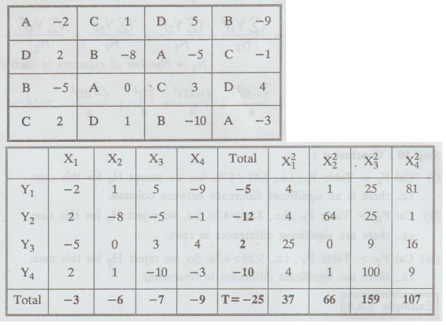
A farmer wishes to test the effects of four different fertilizers A, B, C, D on the yield of wheat. In order to eliminate sources of error due to variability in soil fertility, he uses the fertilizers, in a Latin square arrangement as indicated in the following table, where the numbers indicate yields in bushels per unit area.

Perform an analysis of variance to determine, if there is a significant difference between the fertilizers at a = 0.05 level of significance. [A.U. M/J 2007] [Tvli M/J 2009] [A.U N/D 2012] [A.U A/M 2019 R-17] [A.U N.D 2020 R-17]

Solution :

Subtract 20 we get

H₀ : There is no significant difference between rows, columns and treatments.

H₁ : There is significant difference between rows or columns or treatments.

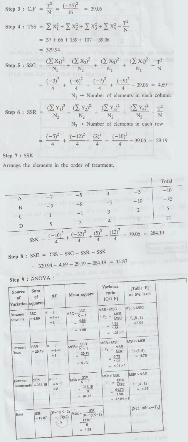
Step 1: N = 16

Step 2: T = -25

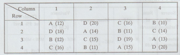
Step 10 : Conclusion :

(i) Cal Fe < Table Fe i.e., 1.27 < 8.94. So, we accept Ho for this case.

i.e., there is no significant difference between the columns.

 (ii) Cal F_T > Table F_T i.e., 4.91 > 4.76. So, we reject Ho for this case.

i.e., there are significant differences in rows.

(iii) Cal F_R > Table F_R i.e., 47.84>4.76. So, we reject Ho for this case. i.e., there are significant differences in treatments.

 

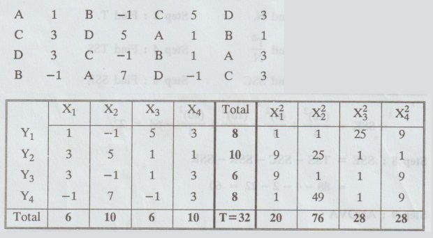
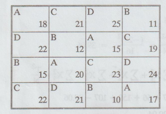
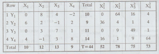
Example 2.4.4

Illustration: Analyse the following of Latin square experiment. [A.U Tvli. M/J 2011, A.U. M/J 2012, M/J 2013]

The letters A, B, C, D denote the treatments and the figures in brackets denote the observations.

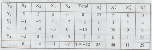
Solution: Let us take 12 as origin for simplifying the calculations.

H₀ : There is no significant difference between rows, columns and treatments.

H₁ : There is significant difference between rows or columns or treatments.

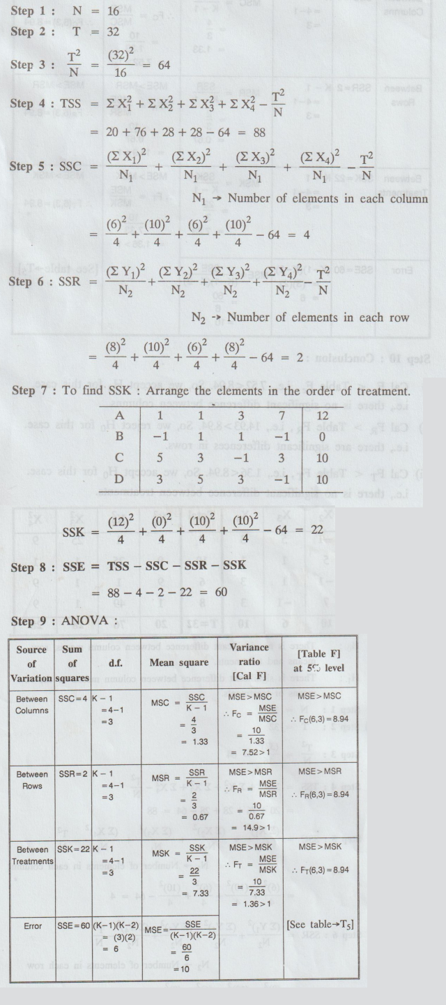
Step 1: N = 16

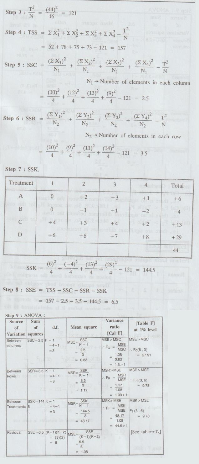
Step 2: T = 44

Step 10: Conclusion :

(i) Cal Fe < Table Fe  i.e., 1.3 < 27.91. So, we accept H₀ for this case.

i.e., there is no significant difference between the columns.

(ii) Cal F_R < Table F_R i.e., 1.08 < 9.78. So, we accept H₀ for this case.

i.e., there is no significant difference between the rows.

(iii) Cal F_T > Table F_T i.e., 44.6 > 9.78. So, we reject H₀ for this case.

i.e., there are significant differences in treatments.

 

Example 2.4.5

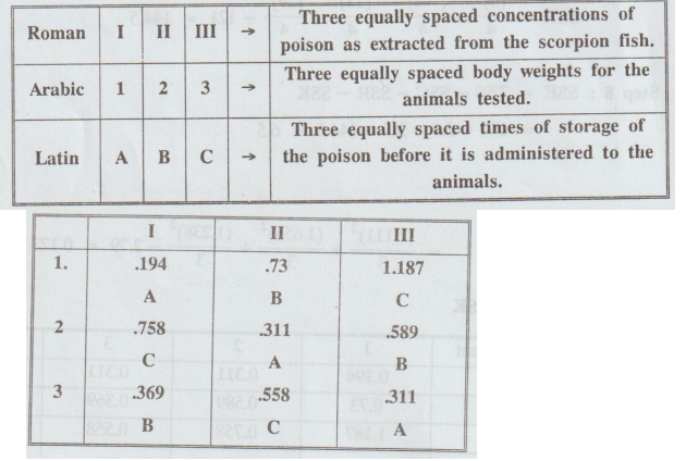
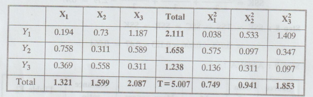
Perform Latin Square Experiment for the following:

Solution :

H₀ : There is no significant difference between rows, columns and treatments.

H₁ : There is significant difference between rows or columns or treatments.

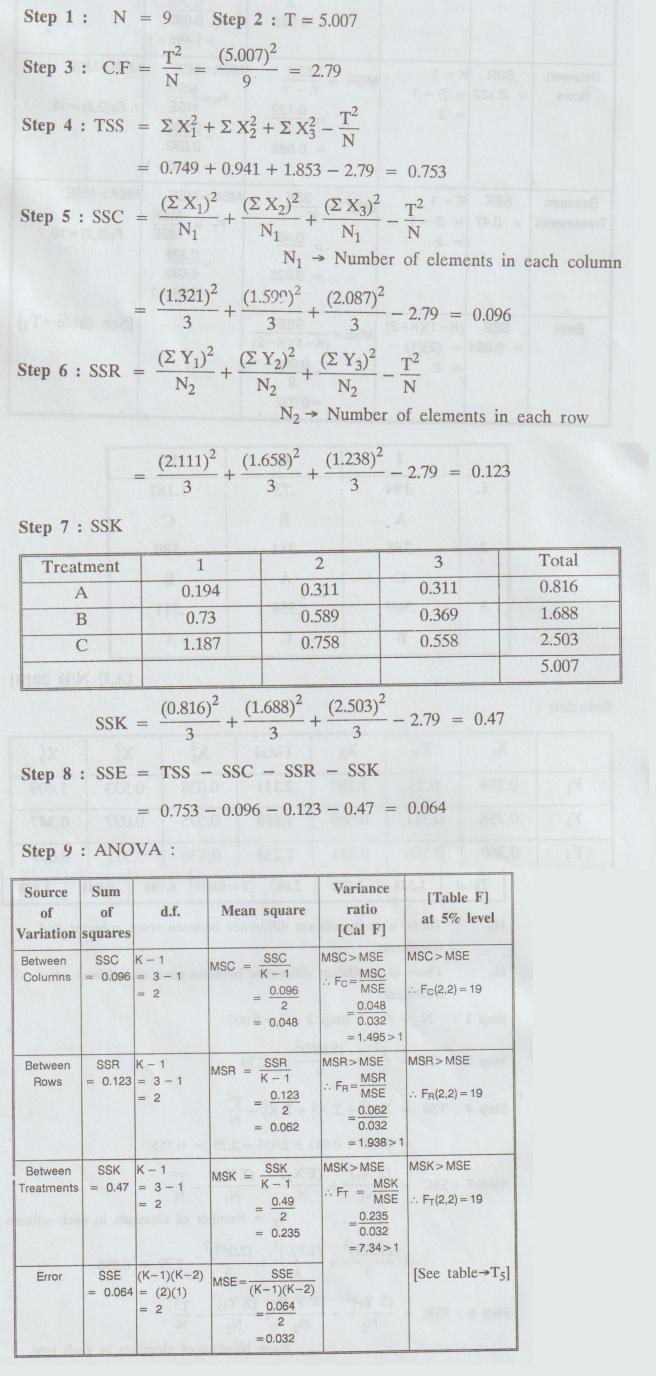
Step 10 : Conclusion:

(i) Cal Fe < Table Fe, i.e., 1.495 < 19. So, we accept H₀ for this case.

i.e., there is no significant difference in columns.

(ii) Cal F_R Table F_R, i.e., 1.938 < 19. So, we accept H₀ for this case.

i.e., there is no significant difference in rows.

(iii) Cal F_T < Table F_T, i.e., 7.34 < 19. So, we accept Ho for this case.

i.e., there is no significant difference in treatments.

 

Example 2.4.6

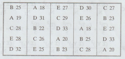
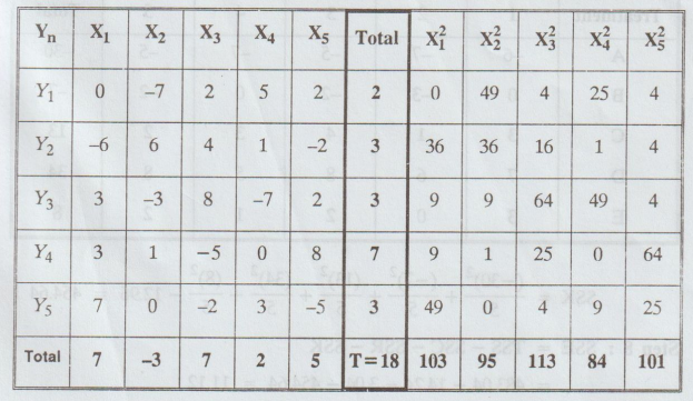
In a Latin square experiment given below are the yields in quintals per acre on the paddy crop carried out for testing the effect of five fertilizers A, B, C, D, E. Analyze the data for variations.

Solution :

It is a 5 × 5 Latin square. Let us subtract 25 from all the items.

H₀ : There is no significant difference between rows, columns and  treatments.

H₁ : There is significant difference between rows or columns or treatments.

Step 1: N = 25

Step 2: T = 18

Step 10 Conclusion :

(i) Cal Fe Table Fe, i.e., 3.84 > 3.26. So, we reject H₀ for this case.

i.e., there are significant differences in columns.

(ii) Cal F_R < Table F_R, i.e.,1.22 < 5.91. So, we accept H₀ for this case.

i.e., there is no significant difference between rows.

 (iii) Cal F_T > Table F_T, i.e., 122.61 > 3.26. So, we reject Ho for this case.

i.e., there are significant differences in treatments.

 

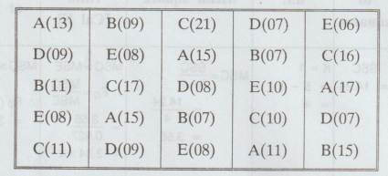
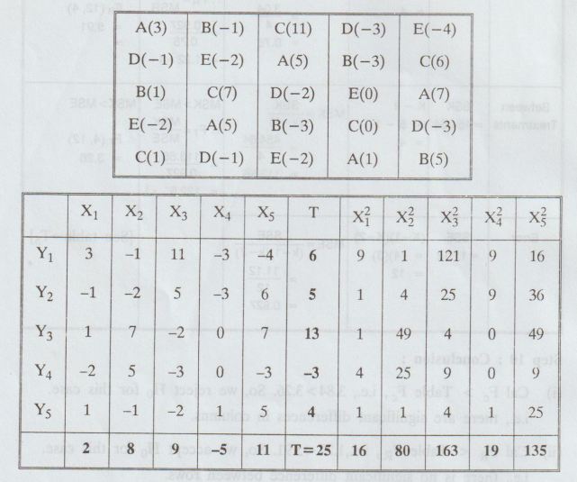
Example 2.4.7

Analyze the data given below and interpret the results.

Solution

Subtract 10 from the given data

H₀ : There is no significant difference between column means, row means and treatments.

H₁ : There is significant difference between column means or the row means or treatments.

Step 1: N = 25

Step 2: T = 25

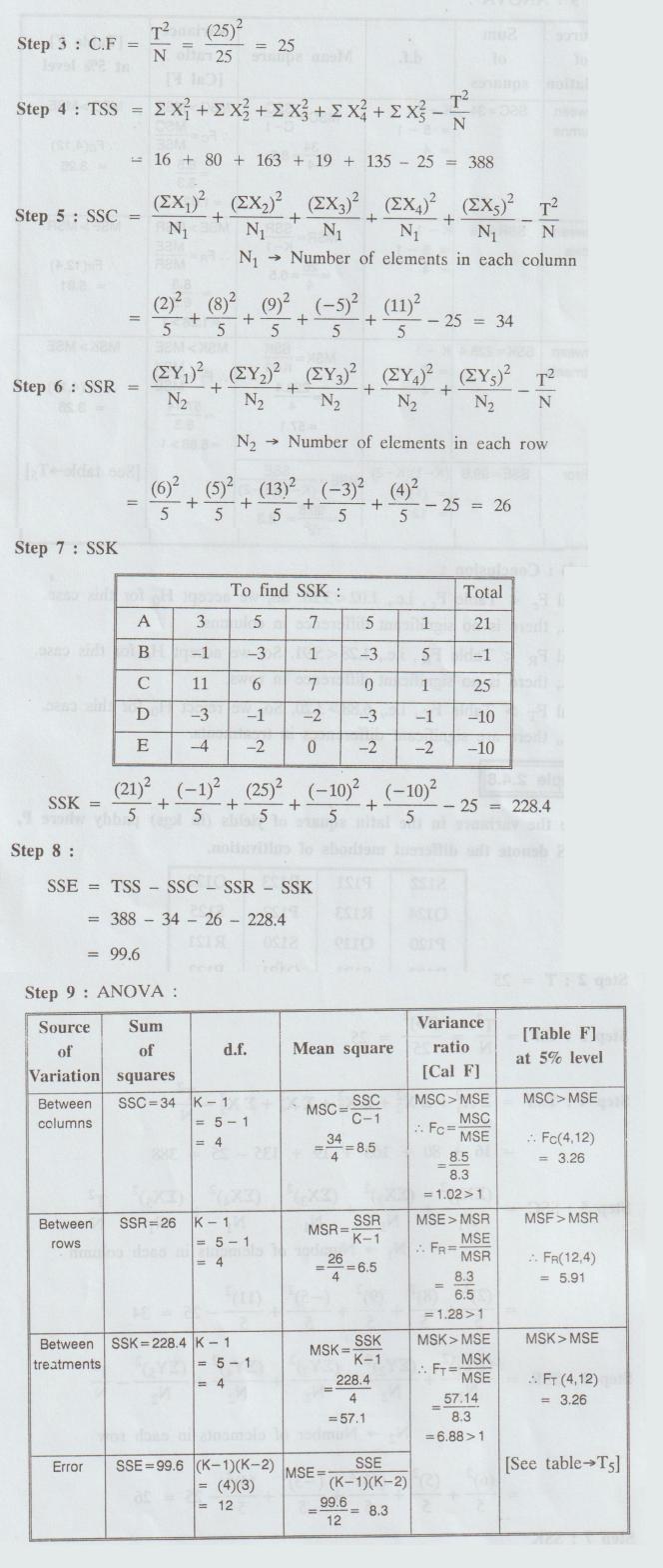
Step 10 Conclusion :

(i) Cal Fe < Table Fe, i.e., 1.02 < 3.26. So, we accept Ho for this case.

i.e., there is no significant difference in columns.

(ii) Cal F_R < Table F_R, i.e., 1.28 < 5.91. So, we accept Ho for this case.

i.e., there is no significant difference in rows.

(iii) Cal F_T > Table F_T, i.e., 6.88 > 3.20. So, we reject Ho for this case. i.e., there are significant differences in treatments.

 

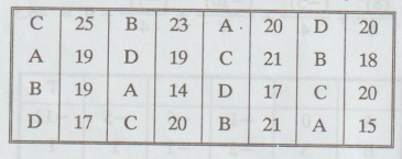
Example 2.4.8

Analyze the variance in the latin square of yields (in kgs) paddy where P, Q, R, S denote the different methods of cultivation.

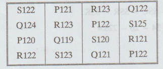
Examine whether the different methods of cultivation have given significantly different yields.so lo Tobro odini atasmala adi sgantA [A.U. N/D 2003, M/J 2006, N/D 2012] [A.U N/D 2019 R-17]

Solution . Subtract 120 weget

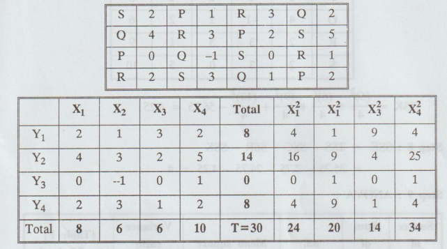
H₀ : There is no significant difference between rows, columns and treatments.

H₁ : There is significant difference between rows or columns or treatments.

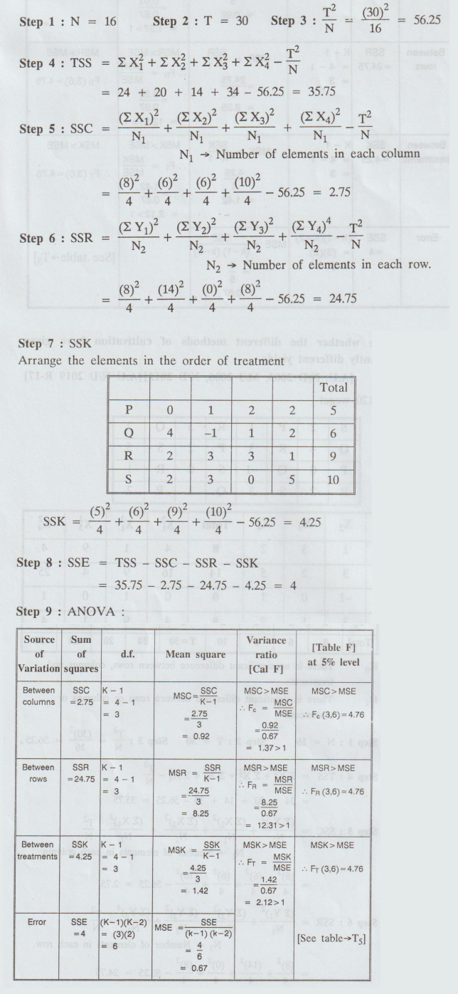
Step 10 Conclusion :

(i) Cal Fe < Table Fc, i.e., 1.37 < 4.76. So, we accept Ho for this case.

i.e., there is no significant difference in columns.

(ii) Cal F_R > Table F_R, i.e., 12.31 >4.76. So, we reject Ho for this case.

i.e., there are significant differences in rows.

(iii) Cal F_T < Table F_T, i.e., 2.12 < 4.76. So, we accept Ho for this case.

i.e., there is no significant difference in treatments.

 

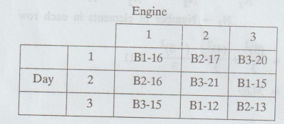
Example 2.4.9

The following data resulted from an experiment to compare 3 burners B1, B2, B3. A Latin square design was used as the tests were made on 3 engines and were spread over 3 days. Perform an analysis of variance at 5% level of significance on the data.

Solution :

H₀ : There is no significant difference between rows, columns and treatments.

H₁ : There is significant difference between rows or columns or treatments.

Subtract 16 from each figure

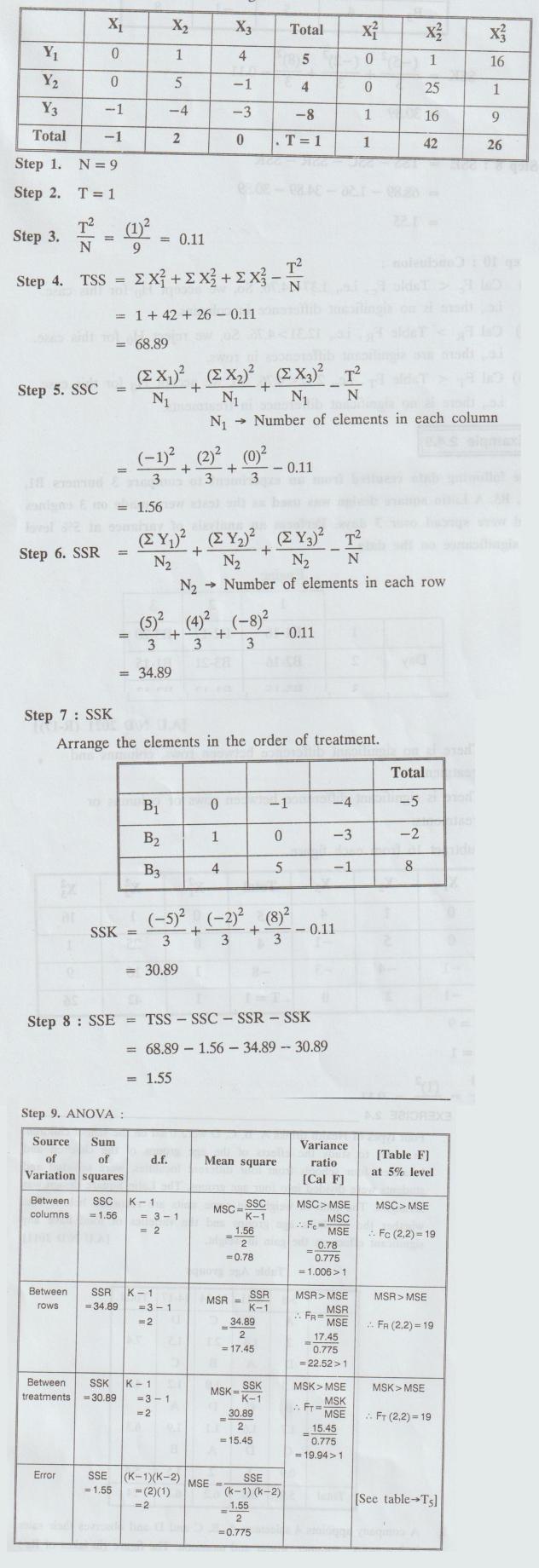
Step 10 Conclusion :

(i) Here, Cal Fc < table Fe i.e., 1.006 < 19

So, we accept H₀ for this case.

i.e., there is no significant difference between columns.

(ii) Here, Cal F_R > table F_R i.e., 22.52 > 19

So, we reject Ho for this case.

i.e., there are significant differences in rows.

(iii) Here, Cal F_T > table F_T i.e., 19.94 > 19

So, we reject Ho for this case.

i.e., there are significant differences in treatments.