Medium Transmission line

Medium Transmission line

AU : Nov.-04, April-96, 98, 99, 2000, Dec.-09, 13, 15, 16, May-05, 09, 11,12,13,14,16,18

The short transmission lines have smaller lengths and the power transmitted by these lines are comparatively at lower voltages. Due to this, while analysing short transmission lines, the effect of capacitance is neglected. With increase in length and voltage of transmission line, the capacitive effects are dominant and they can not be neglected.

The medium transmission lines are having length lying between 50 to 150 km and they operate at voltage greater than 20 kV. Hence in making the analysis of medium transmission line, we have to take into account the effect of capacitance for better accuracy.

The capacitance is uniformly distributed along the length of transmission line. For the simplicity in the calculations, the line capacitance is assumed to be limped at one or more points. This is known as localising of line capacitance and it gives fairly accurate results. The various methods that uses localising of line capacitance are

i) End condenser method ii) Nominal T method iii) Nominal π method

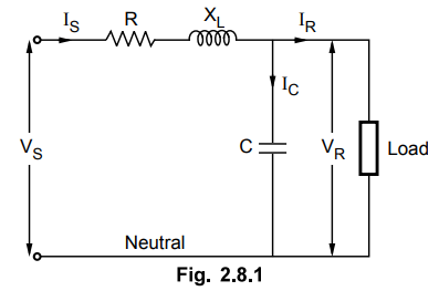
1. End Condenser Method

In this method the line capacitance is lumped or concentrated near the load or at the receiving end. This method overestimates the effect of capacitance.

In case of 3 phase systems, it is always convinient to represent a single phase instead of line to line values. Fig. 2.8.1 shows one phase of three phase transmission line.

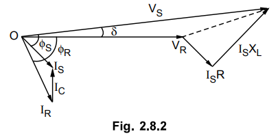
The corresponding phasor diagram shown in the Fig. 2.8.2.

Let V_S = Sending end voltage

V_R = Receiving end voltage

I_R = Load current per phase

X_L = Inductive reactance per phase

C = Capacitance per phase

cos ϕ_R = Receiving end power factor

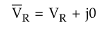
As V_R is the reference vector,

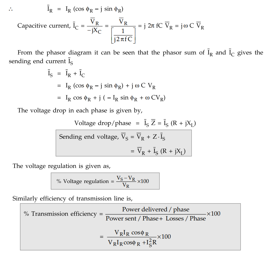
The load current I_R is lagging behind V_R by an angle of ϕ_R

It can be seen that this method is having some limitations although this method is simple to operate. The disadvantages are

i) This method assumes the capacitance to be lumped near the receiving end although in actual practice it is distributed along its length. Due to this there is considerable error of about 10 % in the calculations.

ii) The effects of line capacitance are overestimated in this method.

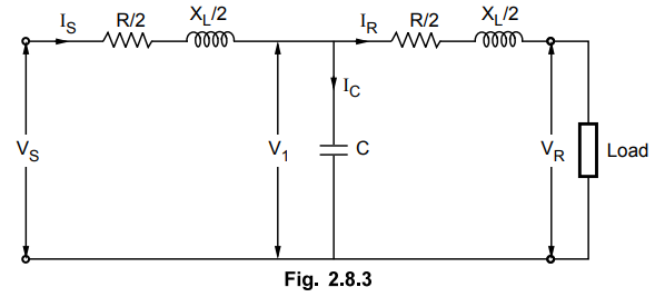
2. Nominal T Method

This method is used for the analysis of medium transmission line. In this method the total line capacitance is lumped or concentrated at the mid point of the line. The resistance and reactance of the line are divided with half the resistance and reactance on 

one side and remaining half on other side of capacitor. Half of the line carries full charging current with this arrangement. Fig. 2.8.3 shows the arrangement used in nominal T method for one phase. It is desirable to work in phase instead of line values.

The corresponding phasor diagram is represented in the Fig. 2.8.4.

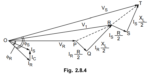
Here the receiving end voltage VR is taken as reference. The drop PQ (I_R . R / 2) is phase with IR. The drop QR (I_R . X_L / 2) is leading I_R by 90^o. The phasor sum of these drops with V_R gives the voltage V₁ which is the voltage across the capacitor. The capacitor current leads V_C by 90°. The phasor sum of I_R and gives I_S. The drop Rg f IS •Ris in phase with Ig whereas drop ST (I_S . X_L / 2) is leading Is by 90°. The phasor sum of these drops along with V₁ gives the sending end voltage V_S.

Sum of these drops along with V₁ gives the sending end voltage V_S

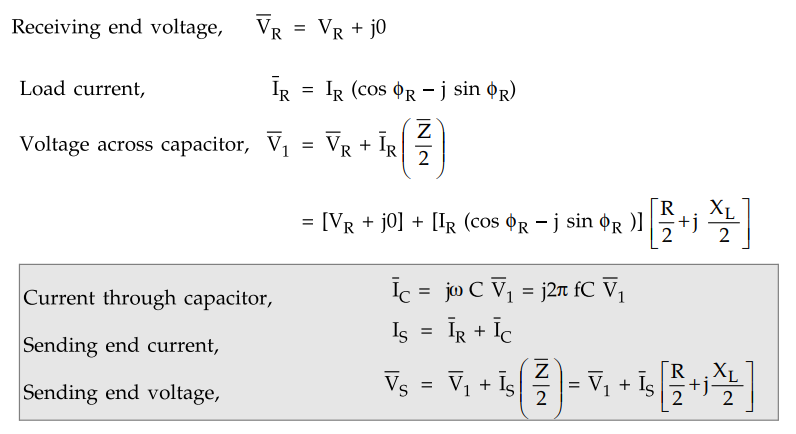
Let     I_R = Receiving end load current per phase

R = Resistance per phase, X_L = Inductive reactance

C = Capacitance per phase, cos ϕ_R = p.f. at receiving end

V_S = Sending end voltage, V₁ = Voltage across capacitor

The efficiency and regulation can be calculated in the similar manner explained in earlier sections.

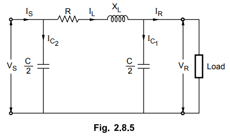
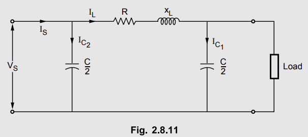
3. Nominal π Method

This is also a localised capacitance method in which capacitance is divided into two halves with one half lumped near sending end and other half near the receiving end. This is shown in the Fig. 2.8.5. The capacitor near the sending end does not contribute any line voltage drop but it should be added with line current to get total sending end current. For convenience and simplicity in calculations only one phase out of three phases is shown.

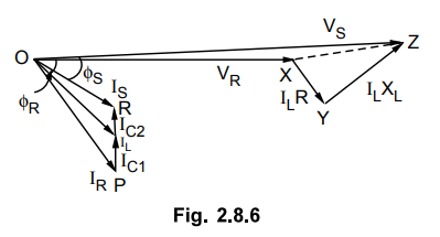
The corresponding phasor diagram is shown in the Fig. 2.8.6 VR is taken as the reference phasor. The current  lags behind V_R by angle ϕ_R. The current through capacitor C₁ is leading the voltage V_R by an angle of 90°. The phasor sum of I_R and I_C1 gives the line current I_L. The drop I_LR is in phase with I whereas drop I_LX_L is leading by 90°. The phasor sum of these drops with V_Ŕ gives the sending end voltage Vs. The capacitor current I_C2 is leading voltage V_S by 90°. The phasor sum of I_S and I_C2 gives the sending end line current I_S.

Let     V_S = Sending end voltage, V_R = Receiving end voltage

I_R = Load current or receiving end current

R = Resistance per phase,

X_L = Inductive reactance per phase

C = Capacitance per phase, cos ϕ_R = p.f. at receiving end

The efficiency and the regulation of the transmission line can be obtained in the similar manner as explained in the earlier sections.

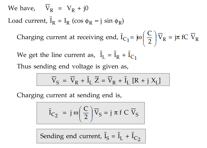
Example 2.8.1 A 3 ϕ, 50 Hz, 100 km line has the following constants.

Resistance/phase/ km = 0.153 ohm, inductance / phase / km = 1.21 mH, capacitance/phase I km = 0.00958 pF. If the line supplies a load of 20 MW at 0.9 pf lagging at 110 kV at the receiving end calculate sending end current, sending end power factor, regulation and transmission efficiency using nominal T method.

Solution : Total line length = 100 km

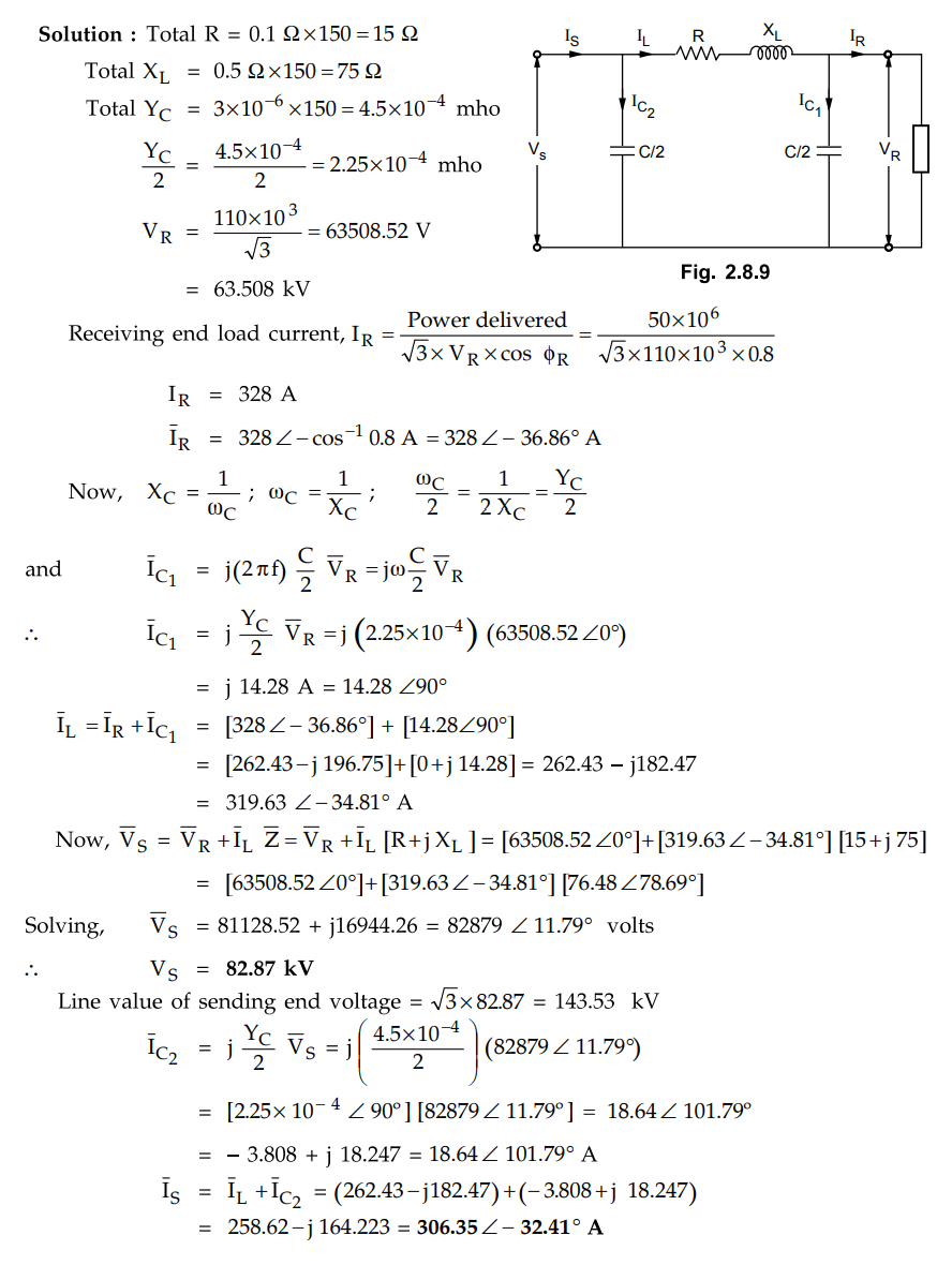
Example 2.8.2 A 50 Hz three - phase transmission line is 150 km long and delivers 50 MW at 0.8 p.f. lag and at 110 kV. The resistance and reactance of the line per conductor per kilometre are 0.1 ohm and 0.5 ohm respectively. The line charging admittance is 3 x 10 ~ 6 mho/km per phase. Compute by apply nominal n method, sending end voltage and current. 

Solution :

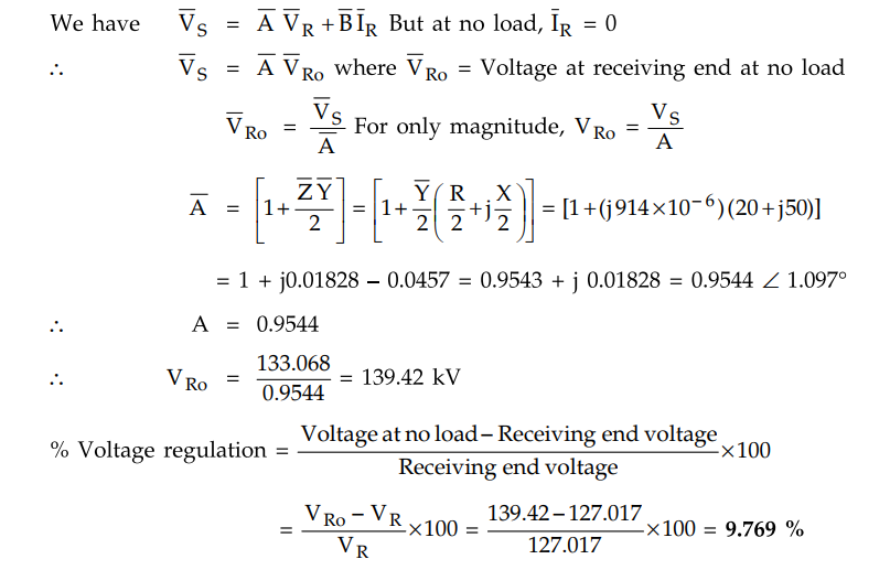
Voltage regulation is nothing but change in voltage at receiving end from no load to full load.

Example 2.8.2 A 3-phase, 50 Hz, transmission line is 150 km long and deliver 50 MW at 0.8 p.f. lag and at 110 kV. The resistance and reactance of the line per conductor per kilometer are 0.1 ohm and 0.5 ohm respectively. The line charging admittance is 3 × 10-6 mho/km per phase. Compute by apply nominal π method, sending end voltage and current.

Solution :

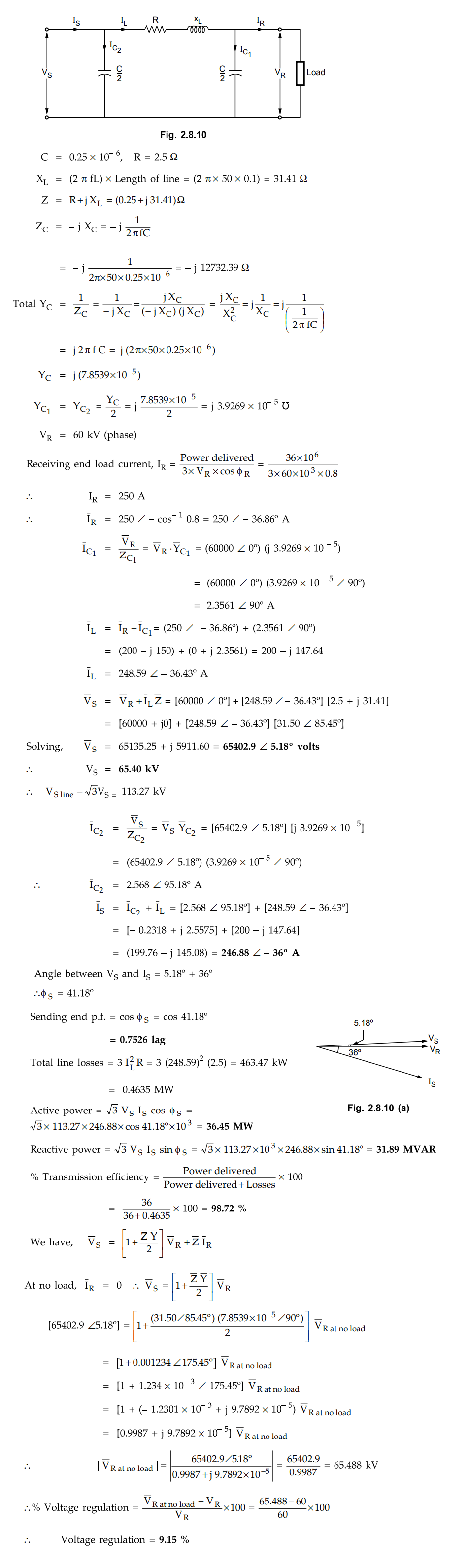
Example 2.8.4 A 3-phase, 50 Hz, 40 km long overhead line has the following line constants : resistance per conductor = 2.5 ohm, inductance per conductor = 0.1 H, capacitance per conductor = 0.25 pF. The line supplies a load of 36 MW at 0.8 power factor lagging at a voltage of 60 kV (phase) at the receiving end. Use nominal n representation, calculate sending end voltage, sending end current, sending end power factor, regulation and efficiency and active and reactive voltamperes.

Solution :

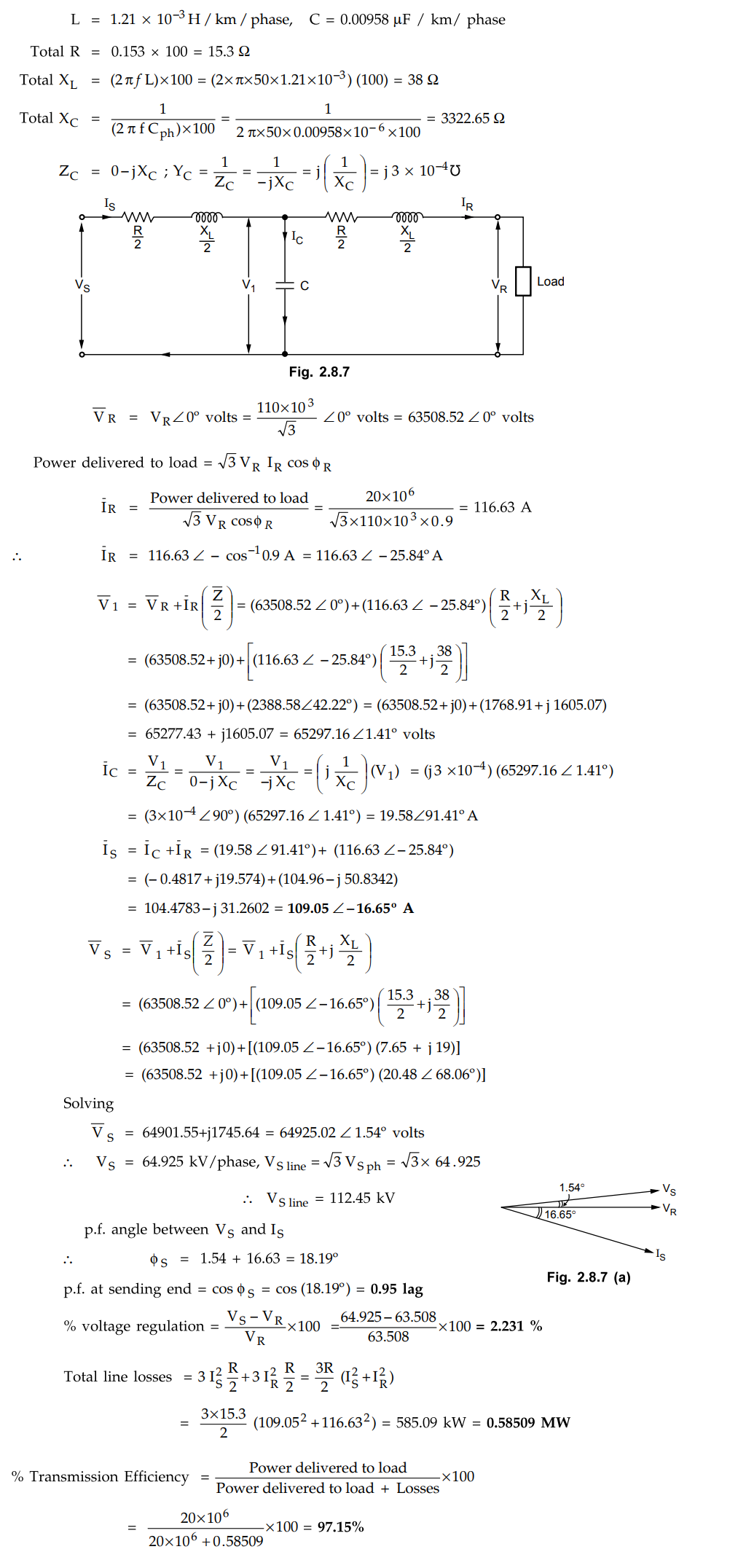
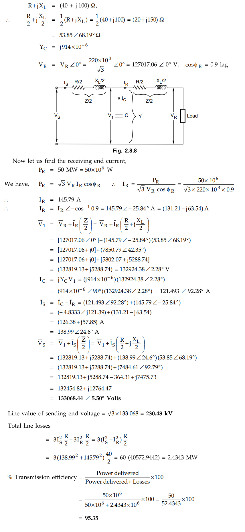
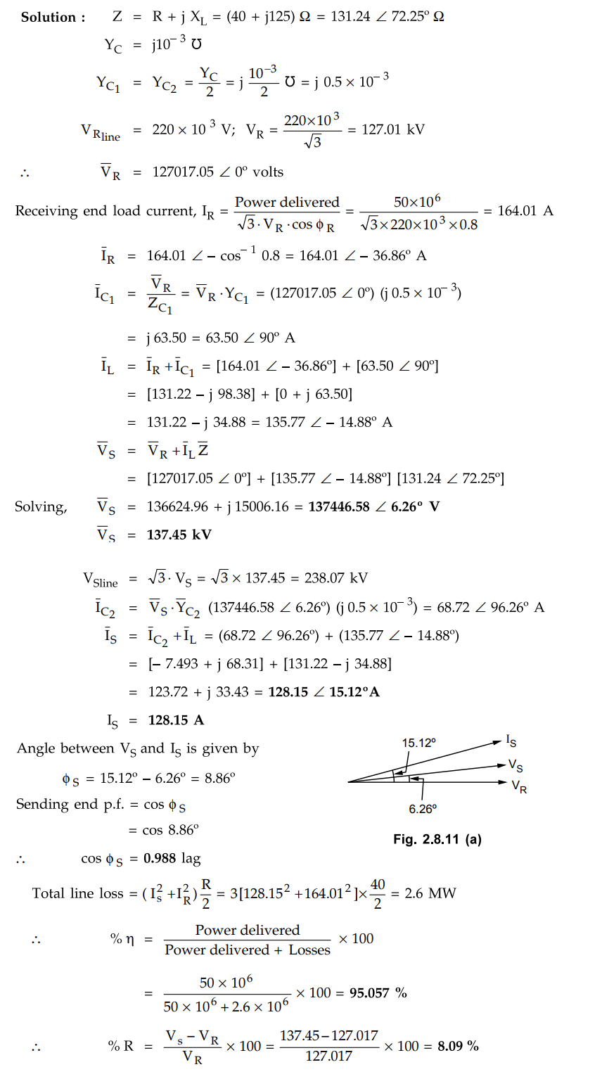
Example 2.8.5 A 50 Hz, 3 phase transmission line 30 km long has a total series impedance of (40+ j 125) ohm and shunt admittance of 10^-3 mho. The load is 50 MW at 220 kV with 0.8 lagging power factor. Find the sending end voltage, current and power factor. Use nominal method. Also find efficiency and regulation.

AU Dec.-09, 16, Marks 16

Solution : 

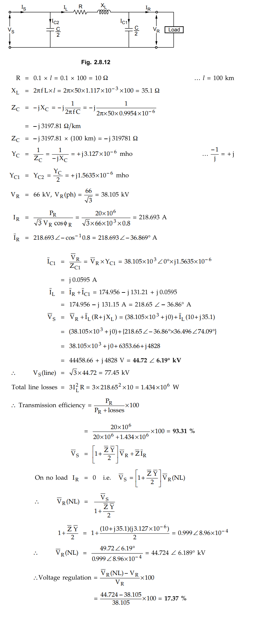
Example 2.8.6 Determine the efficiency and. regulation of a 3-phase, 100 km 50 Hz transmission line delivering 20 MW at a.pf. of 0.8 lagging and 66 kV to a balanced load. The conductors are of copper, each having resistance 0.1 ohm per km, inductance 1.117 mH per km and capacitance 0.9954 pF per km. Neglect leakage and use nominal π-method.

Solution : The nominal n circuit is shown in the Fig. 2.8.12.

Review Questions

1. Derive the expressions for sending end voltage and current of a medium transmission line nominal T-method interms of Y, Z, V_R and I_R.

2. Determine the sending end voltage and sending end current for medium transmission lines, assuming nominal n method.

3. Explain with vector diagram the nominal T method for obtaining the performance calculations of medium transmission lines.

4. A 3 phase 50 Hz overhead transmission line has the following constants per phase R = 28 Ω, X = 63 Ω, ɤ = 4 × 10^-4 (Ʊ). If the load at the receiving end is 75MVA at 0.8 pf. lag with 132 kV between lines, calculate the voltage, current and pf. at the sending end. Use nominal π method.

[Ans: 95.67 kV, 306.73 A, 0.7785 lag]

5. A three phase 50 Hz transmission line is 150 km long and delivers 25 MW at 0.85 pf. lag and at 110 kV. The resistance and reactance of the line per conductor per kilometre are 0.3 ohm and 0.9 ohm respectively. The line charging admittance is 3 ×10^-5 mho/km per phase. Compute by apply nominal n method a) Voltage regulation and b) Efficiency.     

[Ans.: 1.5 %, 89.92 %] 

6. A 66 kW, 3 phase transmission line 160 km long has the following constants Resistance per km = 0.156 ohm, Reactance per km = 0.5 ohm, Susceptance per km = 8.75 × 10^-6 mho

If the line supplies a load of 15 MW at 0.8 pf lagging at 66 kV at the receiving end, calculate sending end voltage, current and power factor using a) Nominal T method b) Nominal n method.

AU : April-2000

7. Determine the sending end voltage for the following, using Nominal method. The transmission line is 120 km long and delivers 40 MW at 132 kV and 0.8 p.f. lagging.

AU: May-05, Marks 8 

[Ans.: 149.87 kV]

8. Explain the following methods for medium transmission lines.

i) End condenser method ii) Nominal T method (middle condenser method)

AU : May-13, Marks 16

9. A 3 phase, 50 Hz, 100 km transmission line has the following constants

Resistance I phase / km = 0.1 Ω

Reactance / phase / km = 0.5 Ω

Susceptance / phase / km = 10^-5 mho

If the line supplies a load of 20 MW at 0.9 pf. lagging at 66 kV at the receiving end calculate by using nominal π method

i) Sending end current ii) Line value of of sending end voltage iii) Sending end power factor iv) Transmission efficiency.

[Ans.: 176.50 A, 76 kV, 0.9057 lag, 95.02%]

10. Explain the end condenser method for medium transmission lines.