Normal distributions

NORMAL DISTRIBUTIONS

The Normal Distribution was introduced by the French Mathematician Abraham De Moivre in 1733. Demoivre, who used this distribution to approximate probabilities connected with coin tossing, called if the exponential bell-shaped curve.

1. Normal Distribution

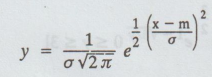
A normal distribution is a continuous distribution given by

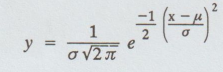
where X is a continuous normal variate distributed with density function 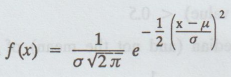 with mean μ and standard deviation σ

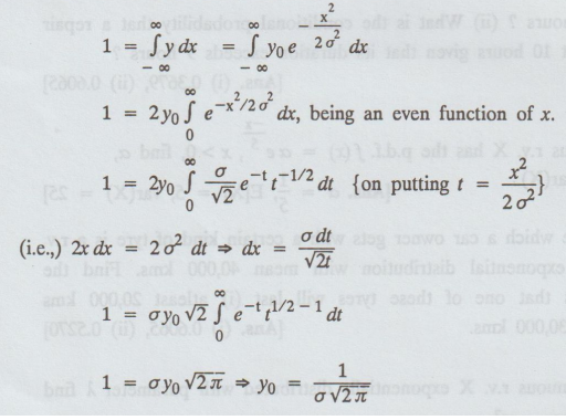
2. Deviation of the distribution

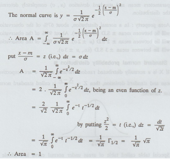
Let the equation of the normal curve be 

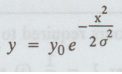
It will be a normal probability curve if

In the above derivation, mean has been taken at the origin, but if however another point is taken as the origin such that the excess of the mean over the arbitrary origin is 'm', then

 is the standard form of the normal curve with origin at (m, 0).

3. Area under the normal curve is unity

4. Characteristics of the Normal Distribution

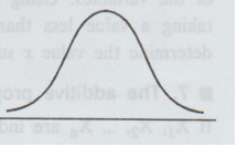
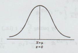
The diagram of a normal distribution is given below. It is called normal curve. It suggests several important properties of the normal distribution.

1. The normal distribution is a symmetrical distribution and the graph of the normal distribution is bell shaped.

2. The curve has a single peak point (i.e.,) the distribution is unimodal.

3. The mean of the normal distribution lies at the centre of normal curve.

4. Because of the symmetry of the normal curve, the median and mode are also at the centre of the normal curve. Hence in a normal distribution the mean, median and mode coincide.

5. The tails of the normal distribution extend indefinitely and never touch the horizontal axes. That is, we say that the normal curve approaches asymptotically on either side of its horizontal axes.

6. The normal distribution is a two parameter probability distribution. The parameters mean and standard deviation (u, o) completely determine the distribution. 

7. Area property: In a normal distrbution, about 67% of the observations

will lie between mean ± S.D (i.e., μ ± σ). About 95% of the observations

will lie between mean ± 2 S.D (μ ± 2σ). About 99% of the observations

will lie between mean ± 3 S.D (i.e., μ ± 3σ).

5. Standard normal probability distribution

If X is a normally distributed random variable μ and σ are respectively its mean and standard deviation, then Z = X - μ /σ is called standard normal random variable.

Special table called table of areas under normal curve is available to determine probabilities that the random variable lies in a given range of values of the variables. Using the table, we can determine the probability for X, taking a value less than x (X < x) and also for a given probability we determine the value x such that X < x.

7. The additive property of Normal Distribution

If X₁, X₂, ... X_n are independent normal variates with parameters

(m₁, σ₁), (m₂, σ₂) (m_n, σ_n) respectively, then X₁ + X₂ +...+ X_n is also a normal variate with parameter (m, σ),

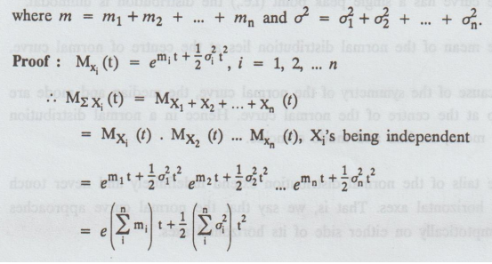
which is the moment generating function of a normal variate with mean

Hence, X₁ + X₂ + ... + X_n follow normal distribution with mean