Poisson distribution: Solved Example Problems

Example 1.8.1

If X is a Poisson variate such that P(X = 2)= 9P(X = 4) + 90P(X = 6), find the variance. [A.U. A/M. 2008, M/J 2013]

Solution: The probability distribution for the Poisson R.V. X is given by,

( λ² + 4 ) (λ² – 1) = 0

λ² = - 4 (or) λ² = 1 ⇒ λ = 1 [λ > 0]

For a Poisson distribution, Var (X) = λ = 1.

 

Example 1.8.2

Write down the probability mass function of the Poisson distribution which is approximately equivalent to B (100, 0.02).

Solution:

Given: n = 100 , p = 0.02,

 λ = np = 100 × 0.02 = 2

Hence, the probability distribution is

x = 0, 1, 2, ...

 

 Example 1.8.3

If X and Y are independent Poisson variate such that P(X = 1) = P(X = 2) and P(Y= 2) = P(Y= 3) X-2Y.

Solution : We know that, P(X = x) = e^-λ λ^x/x!

Given: P(X = 1) = P (X = 2)

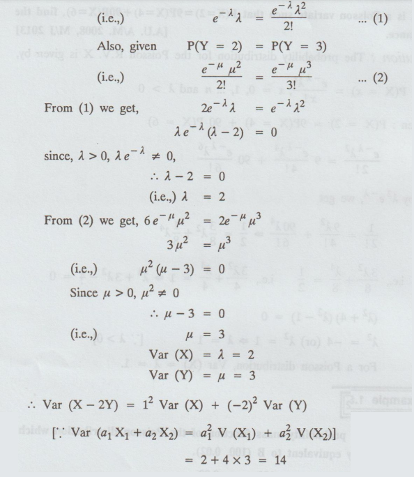
Var (X) =  λ = 2

Var (Y) = μ = 3

 Var (X - 2Y) = 1² Var (X) + (-2)² Var (Y)

[ Var (a₁ X₁ + a₂ X₂) = a₁² V (X₁) + a₂² V (X₂)]

=2+ 4 × 3 = 14

 

Example 1.8.4

What are the main characteristics of the Poisson distribution and give some example of the same.

Solution:

Its main characteristics are:

(i) It is the limiting form of binomial distribution when n is large and p (or q) is small.

 (ii) Here p (or q) is very close to zero or unity, but if p is very close to zero, the distribution is unimodal.

(iii) As it consists of a single parameter ' λ ' the entire distribution can be obtained by knowing the mean ' λ ' only.

Some examples :

(i) The number of defective screws per box of 100 screws.

(ii) The number of typographical errors per page in a typed material.

(iii) The number of cars passing through a certain street in time t'.

 

Example 1.8.5

Is the additive or reproductive property of Poisson distribution true for (i) the mean of two Poisson variates (ii) the difference between the two independent Poisson variates.

Solution: (i) The mean of two Poisson variates cannot be a Poisson variate, since the average can take fractional values which are not possible for a Poisson variate.

(ii) The difference between the independent Poisson variates is not a Poisson variate; because, the difference can take negative values also, whereas in a Poisson distribution, negative values are not permitted.

 

Example 1.8.6

Deduce the mean and four moments of the Poisson distribution from binomial distribution as a limiting case : [A.U A/M 2019 (R17) RP]

Solution : Binomial distribution → Poisson distribution, when n→ ∞, np = λ and p or q→ 1

Mean of binomial distribution np = λ

= mean of Poisson distribution

µ₂ (for binomial distribution) = npq → np = λ = μ₂  (for Poisson distribution) as q→ 1.

μ₃ (for binomial distribution) = npq (q - p)

→ np (1 - p) as q→ 1

→ npq → np = λ = µ₃ (for Poisson distribution)

µ₄ (for binomial distribution)

= npq [1+ 3 (n - 2) pq ] → np (1 + 3 np) as p→ 0, q→ 1

λ + 3λ₂ =μ₄ (for Poisson distribution)

Example 1.8.7

If X and Y are independent Poisson variates, show that the conditional  distribution of X given X + Y is binomial. [A.U. M/J 2006]

Solution: X and Y are independent Poisson variates with parameter λ₁ and λ₂ respectively

 X + Y is a Poisson variate with parameter λ₁+ λ₂.

X = r X+Y=n

 [ X and Y have Poisson distribution with parameters λ₁ and λ₂  ⇒ X + Y also has Poisson distribution with parameter λ₁ + λ₂]

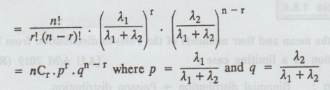
= pdf of binomial distribution.

Hence the result.

 

Example 1.8.8

The sum of two independent Poisson variates is a Poisson variate. [A.U. M/J 2006] [A.U N/D 2018 R-17 PS]

Solution: Let X₁, X₂ be the two independent Poisson variate with parameter λ₁ , λ₂ respectively.

Now, M_{X1 + X2} (t) = M_X1(t) M_x2 (t)

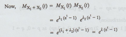
The sum of two independent poisson variates is a Poisson variate.

 

Example 1.8.9

If X₁ and X₂ is independent Poisson variates, show that X₁ - X₂ is not a Poisson variate. [A.U M/J 2006]

Solution: Let X₁, X₂ be the two independent Poisson Variates with parameter λ₁, λ₂ respectively.

Now, M_X1-X2(t) = M_X1(t).M_-X2 (t)

= M_X1 (t). M_X2(-t)

=e^{λ1 (et-1)} e^λ₂ (e^-t-1)

which cannot be expressed in the form of e^{λ(et -1)}

 X₁ - X₂ is not a Poisson variate.

 

Example 1.8.10

Derive the Poisson distribution as a limiting case of Binomial distribution. (OR) State the conditions under which the Poisson distribution is a limiting case of the Binomial distribution and show that under these conditions the binomial distribution is approximated by the Poisson distribution. [A.U N/D 2013, N/D 2014]

Solution: The Binomial probability law for x successes in a series of 'n' independent trials is

P[X = x] = p(x) = nC_xp^x q^{n - x}, x = 0, 1, 2, ... n

To consider it under limiting case when

(i) n is indefinitely large (i.e.,) n→ ∞

(ii) p is very small s.t. p → 0

(iii) np = λ (a finite quantity)

p = λ/n and q = 1− p = 1 – λ/n

P[X ≤ x] = n C_xp^x q^{n - x}

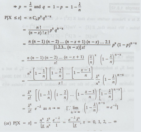
where λ is known as the parameter of the distribution.

 

Example 1.8.11

If X is a Poisson variate such that 2 P[X= 0] + P [X = 2] = 2P [X = 1], find E[X].

Solution:

4 + λ² = 4 λ

λ² - 4 λ + 4 =  0

 ⇒ (λ = 2)² ⇒ λ = 2 ⇒ λ = E[X] = 2

 

Example 1.8.12

If X is a Poisson variate such that E [X²] = 6, then find E[ X]

Solution: We know that, E [X] Var[X] = 2, Given E [X²] = 6

Var[X] = E[X²]-[E(X)²

λ  = 6 - λ² ⇒ λ² +λ = 6

⇒ λ² + λ – 6 = 0

(λ + 3 ) (λ – 1) = 0 ⇒ λ = -3, λ = 2

E[X] = λ = 2 [ λ > 0 ] 

Example 1.8.13

If X is a Poisson variate such that P [X= 0]= 0.5, then find Var[X]

Solution: Given: P [X=0] = 0.5 V

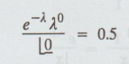
⇒ e^-λ = 0.5

log e^-λ = log(1/2) ⇒ -λ =  − log(1/2)

⇒ λ = log 2

Var(X) = λ =log 2

 

Example 1.8.14

It is known that the probability of an item produced by a certain machine will be defective is 0.05. If the produced items are sent to the market in packets of 20, find the number of packets containing atleast, exactly and atmost 2 defective items in a consignment of 1000 packets using (i) Binomial distribution, (ii) Poisson approximation to Binomial distribution. [A.U Trichy M/J 2011, CBT N/D 2011] [A.U N/D 2017 (RP) R-08]

 Solution: (i) Binomial distribution: Let X denotes the number of defective items produced by a certain machine.

Then P (X = x) = nC_xp^x q^{n -x}, x → 0, 1, 2, ... n

P  → Probability that an item to be defective = 0.05 and q= 0.95 and n = 20.

(a) Number of packets containing atleast 2 defective items = NP(X≥2)

= 1000 [1 - P (X < 2)] =1000 [1 − (P (X = 0) + P(X = 1))]

=1000 [1 − (20C₀ (0.05)⁰ (0.95)²⁰+ 20C¹ (0.05)1 (0.95)¹⁹)] ≈ 264.

(b) Number of packets containing exactly 2 defective items

N [P(X = 2)]

=  1000 [20C₂ (0.05)² (0.95)¹⁸] ≈ 189

 (c) Number of packets containing atmost 2 defective items

= N (P(X ≤ 2))

= N [P(X = 0) + P(X = 1) + P(X = 2)]

= 1000 [20C₀ (0.05)⁰ (0.95)²⁰+ 20C¹ (0.05)¹ (0.95)¹⁹ + 20C₂ (0.05)² (0.95)¹⁸] ~ 925

(ii) Poisson distribution : Since p = 0.05 is very small and n = 20 is sufficiently large, Binomial distribution may be approximated poisson distribution with parameter λ -= np = 20 × 0.05 =1

 

 (a) Number of packets containing atleast 2 defective items

= NP(X≥2)

=1000 [1 - P (X < 2)] = 1000 [1 - [P (X = 0) + P(X = 1)]]

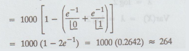
 (b) Number of packets containing exactly 2 defective items

= NP(X=2)

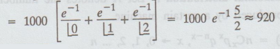
 (c) Number of packets containing atmost 2 defective items

 = NP(X ≤ 2)

=N[P(X = 0) + P(X = 1) + P(X = 2)]

 

Example 1.8.15

If X and Y are independent Poisson variates with means λ₁ and λ₂ respectively,  find the probability that (i) X + Y =K, (ii) X = Y.

Solution :

(i) We know that, for a Poisson variate 'X'

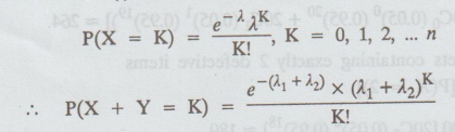
 [By additive property of Poisson distribution]

 (ii) P(X = Y) 

 

Example 1.8.16

If the moment generating function of the R.V is e^4(et-1), then find  P(X = μ+ σ) where μ and σ² are the mean and variance of the Poisson.

Solution:

We know that, for a Poisson distribution, the moment generating function

is M_X(t) = e^{λ(et - 1)}, where λ = 4

Mean = 4 and S.D.= √Var = √4 = 2

P(X = µ + σ ) = P (X = 6)  = 2

P (X = µ + σ ) = P (X = 6) =

 

Example 1.8.17

If X is a Poisson R.V such that P (X = 1) = 0.3 and P (X = 2) = 0.2, then find P (X = 0)

Solution:

If X is a Poisson R.V with parameter λ, then

 

Example 1.8.18

The number of monthly breakdown of a computer is a random variable having a Poisson distribution with mean equal to 1.8. Find the probability that this computer will function for a month.

(1) without a breakdown (2) with only one breakdown and (3) with atleast one breakdown. [AU M/J 2006 MA034] [A.U N/D 2012] [A.U M/J 2007, N/D 2008] [A.U A/M 2017 R-08] [A.U N/D 2017 (RP) R-13]

Solution: Given: mean = λ = 1.8

Let X denotes the no. of breakdowns of a computer in a month.

 (c) P(with atleast 1 breakdown) =P ( X ≥ ) =  1- P(X < 1)

= 1 – P(X = 0 ) = 1- 0.1653 = 0.8347

 

Example 1.8.19(a)

The number of typing mistakes that a typist makes on a given page has a Poisson distribution with a mean of 3 mistakes. What is the probability that she makes

(1) Exactly 7 mistakes = P[X = 7]

(2) Fewer than 4 mistakes = P[X < 4]

(3) No mistakes on a given page = P[X = 0] [A.U N/D 2015 R-8]

Solution: Given: Mean (λ) = 3, P [X = x] = e^-λλ^{x /} x!

(1) P[ X = 7] = e^-3 (3)⁷ / 7! = 0.0216

(2) PX < 4] = P(X = 0] + P(X = 1] + P [X = 2] + P(X = 3]

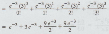
= e⁻³ + 3e^-3 + 9e^-3/2 + 9e^-3/2

= 13e^-3 =(13) (0.0498) = 0.6474

 (3) P [ X = 0] = e^-3(3)⁰ / 0! = e^-3 = 0.0498

 

Example 1.8.19 (b)

The average number of traffic accidents on a certain sections of a highway is two per weak. Assume that the number of accidents follows a Poisson distribution. Find the probability of (i) no accident in a week (ii) atmost two accidents in a 2 week period. [A.U A/M 2019 (R13) RP] [A.U M/J 2009]

Solution: Given: Mean λ = 2 per week

We know that, P [X=x] =  e- ^λ λ^x/x! = e^-2 2^x/x!

(i) P[X = 0] = e^-22⁰/0! = e^-2 = 0.1353

 (ii) During a 2 week period the average number of accidents in this highway 2 + 2 = 4

The probability of atmost two accidents in a 2 week period.

=> P(X ≤ 2) = P[X = 0] + P[X = 1] + P[X = 2]

P[X ≤ 2] = e^-44⁰/0! + e^-4 4¹/1! + e^-44²/2!

= e^-4 [1 +4 +8] = 13 e^-4 = 0.238

 

Example 1.8.20

A book of 500 pages contains 500 mistakes. Find the probability that there are atleast four mistakes per page.

Solution :

Total number of mistakes in Book = 500

Total number of pages = 500

The average of 1 mistake per page i.e., λ = 1

Let X be a random variable mistakes in a page then

 

Example 1.8.21

The atoms of a radioactive element are randomly disintegrating. If every gram of this element, on average, emits 3.9 alpha particles per second, what is the probability that during the next second the number of alpha particles emitted from 1 gm is (a) atmost 6 (b) atleast 2 (c) atleast 3 and atmost 6. [AU N/D 2007]

Solution: Now Mean λ = 3.9

We know that,

 

Example 1.8.22

VLSI chips, essential to the running of a computer system, fail in accordance with a Poisson distribution with the rate of one chip in about 5 weeks. If there are two spare chips on hand, and if a new supply will arrive in 8 weeks. What is the probability that during the next 8 weeks the system will be down for a week or more, owing to a lack of chips? [A.U N/D 2007]

Solution : λ = rate of one chip in about 5 weeks = 1/5

P(system down for atleast one week before new supply in 8 weeks) = P(3 or more failures within 7 weeks)

= 1 - P[0, 1, 2, failures in 7 weeks]

Example 1.8.23

Messages arrive at a switch board in a Poisson manner at an average rate of six per hour. Find the probability for each of the following events:

 (1) exactly two messages arrive within one hour.

(2) no message arrives within one hour

 (3) atleast three messages arrive within one hour.

 [A.U. A/M 2015 R13] [A.U N/D 2016 R13 PQT] [A.U A/M 2018 R-13] [A.U N/D 2017 R-13]

Solution : Mean λ = 6 per hour

We know that P [X = x] = e^-λ λ^x/x! = e^-66^x/x!

(1) P[X=2] = e^-66²/2! = 0.0446

 (2) P[X = 0] = e^-66⁰/0! = 0.0025

 (3) P[X ≥3] = 1-P[X<3]

= 1 - [P [X = 0] + P (X = 1] + P [ X = 2]]

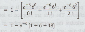
= 1 – e^-6 [1 + 6 + 18]

= 0.9380

 

Example 1.8.24

The probability that a man aged 35 years will die before reaching the age of 40 years may be taken as 0.018. Out of a group of 400 men now aged 35 years, what is the probability that 2 men will die within next 5 years?

Solution : Given that, n = 400 and p = 0.018

λ = np = 0.018 × 400 = 7.2

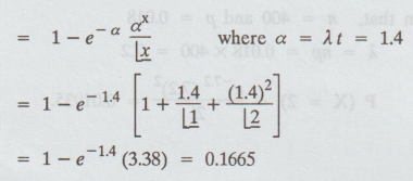
P (X = 2) = e^-7.2 (7.2)²/2! = 0.01935.

 

Example 1.8.25

The manufacturer of pins knows that 2% of his products are defective. If he sells pins in boxes of 100 and guarantees that not more than 4 pins will be defective. What is the probability that a box will fail to meet the guaranteed quality ? vs go galwollol ad! lo doss tol [A.U N/D 2013] [A.U A/M 2018 R8]

Solution : Given that, n = 100 and p = 2% = 2/100

λ = np = 2/100 × 100 = 2

P(X > 4 ) = 1 – P(X ≤ 4 )

 = 1- [P(X = 0)+P(X = 1)+P(X = 2)+P(X = 3)+P(X = 4)]

= 0.05265