Potential Gradient

Potential Gradient

AU : Dec.-07, May-05, 09, 10

• Consider an electric field   due to a positive charge placed at the origin of a sphere. Then,

• The potential decreases as distance of point from the charge increases. This is shown in the Fig. 4.12.1.

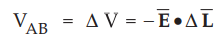
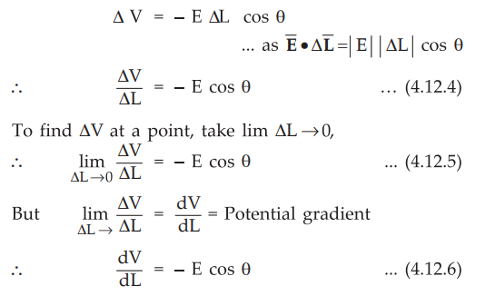
• It is known that the line integral of   between the two points gives a potential difference between the two points. For an elementary length AL we can write,

• Hence an inverse relation namely the change of potential ΔV, along the elementary length ΔL must be related to , as ΔL → 0.

• The rate of change of potential with respect to the distance is called the potential gradient.

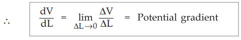
• Potential gradient is nothing but the slope of the graph of potential against distance at a point where elementary length is considered.

• Let us see how this potential gradient is related to the electric field.

1. Relation between   and V

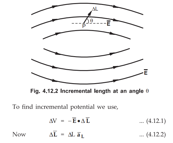
• Consider   due to a particular charge distribution in space. The electric field   and potential V is changing from point to point in space. Consider a vector incremental length  making an angle 0 with respect to the direction of  , as shown in the Fig. 4.12.2.

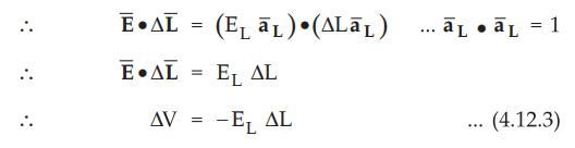
where  = Unit vector in the direction of ΔL.

• Now the dot product means product of magnitudes of one quantity and component of other in the direction of first. So  is the product of component of   in the direction of 

• In other words, dot product can be expressed in terms of cos θ as.

• At a point P where ΔL is considered,   has a fixed value while ΔL is also constant. Hence potential gradient dV/dL can maximum only when cos θ = -1

i.e. θ = +180° This indicates that ΔL must be in the direction opposite to .

dV/dL|max = E  ... (4.12.7)

This equation shows that,

1. Maximum value of the potential gradient gives the magnitude of the electric field intensity  .

2. The maximum value of rate of change of potential with distance i.e. potential gradient is possible only when the direction of increment in distance is opposite to the direction of  .

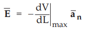
• Thus if  is the unit vector in the direction of increasing potential normal to the equipotential surface then   can be expressed as,

 ... (4.12.8)

• As   and potential gradient are in opposite direction, equation (4.12.8) has a negative sign.

• The equation shows that the magnitude of   is given by maximum space rate of change of V while the direction of E is normal to the equipotential surface in the direction of decreasing potential.

The maximum value of rate of change of potential with distance (dV/dL) is called gradient of V.

• The mathematical operation on V by which –  obtained is called gradient and denoted as

• The equation (4.12.11) gives the relationship between   and V. Now   is vector but V is scalar, hence remember that grad V i.e. gradient of a scalar is a vector.

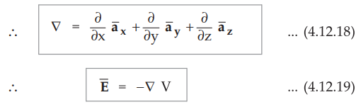
2. The Vector Operator  (del)

• In space the potential V is unique function of x, y and z coordinates, in cartensian system denoted as V (x, y, z). Hence its total differential potential dV can be obtained as,

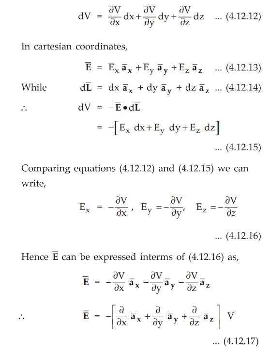
• The potential V is scalar but the operator on V given in equation is vector and is called del operator denoted as . The operation of del on a scalar V is called grad V.

• The gard a scalar is a vector.

• The gard V in various coordinate systems are,

Ex. 4.12.1 An electric potential is given by,

V = (60sin θ / r2) V

Find V and   at P(3,60°, 25°).

AU : Dec.-07, Marks 6

Sol.:

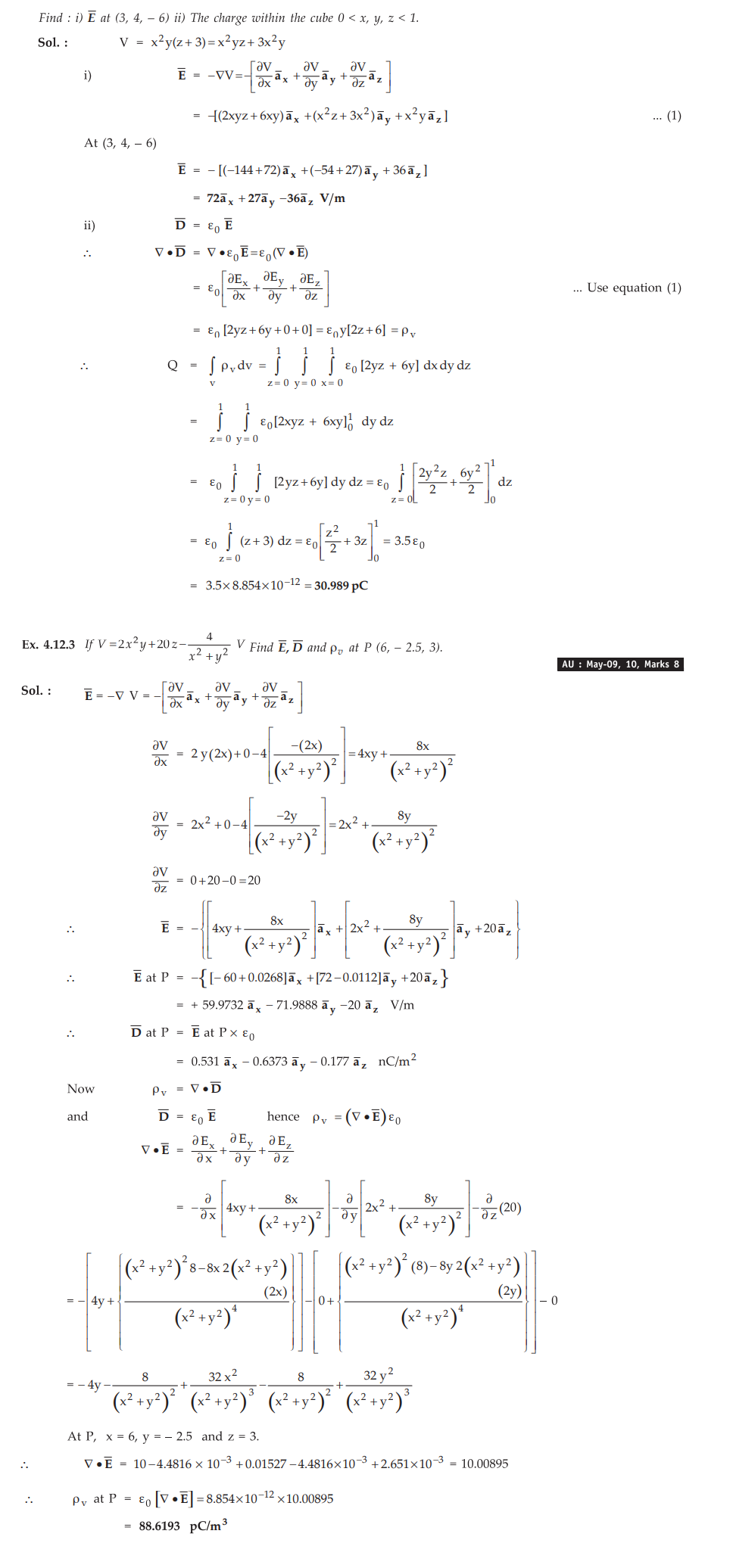
Ex. 4.12.2 In free space V = x2y(z+3)

Find : i)    at (3, 4, - 6) ii) The charge within the cube 0 < x, y, z < 1.

Sol.: 

Ex. 4.12.4 The potential exist in air is V = 10y(x3 + 5) volt, i) Find   at surface y = 0 ii) Show that the surface y = 0 is an equipotential surface, iii) If surface y = 0 is a conductor, find the total charge in the region 0 < x < 2, y = 0, 0 < z < 1. Assume V > 0 in the region outside the conductor.

Sol. :

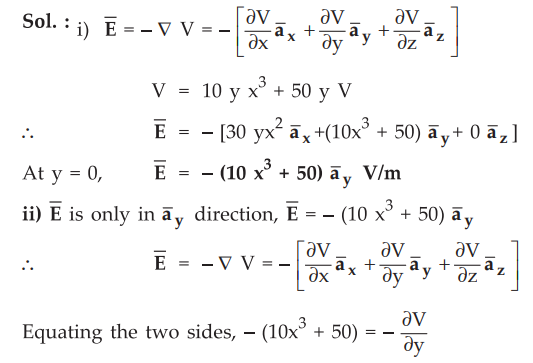
Equating the two sides, - (10x3 + 50) = - ∂V / ∂y

Integrating with respect to y, V = 10x3y + 50 y + C

At y = 0, V = C = Constant

Thus as potential is constant along the surface y = 0,

it is equipotential surface.

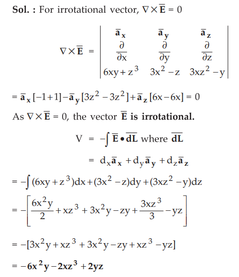
Ex. 4.12.5 Show that the vector

is irrotational and find its scalar potential.

Examples for Practice

Ex. 4.12.6 If the potential field V is V = 100 (x2-y2) find   ,V at a point (2, - 1, 3) and the equation representing the locus of all points having a potential of 300 V.

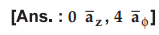
Ex. 4.12.7 Find the rate at which the scalar function V = r2 sin 2ϕ increases in the

i) z direction ii) ϕ direction. Evaluate it at r = 2 m and ϕ = 45 °.

Ex. 4.12.8 Given V = 2x2y - 5z at point P(-4,3,6). find the potential, electric field intensify and volume charge density.

Review Question

1. Define potential gradient and obtain the relation between   and V.