Rigorous Method of Analysis of Long Transmission Line

Rigorous Method of Analysis of Long Transmission Line

AU : May-05, 09, 18, Dec.-05, 06, 12, 13

The Fig. 2.11.1 shows one of the phase out of 3 phases of a long transmission line. The impedance and the shunt admittance of the line are uniformly distributed along the length.

Let us consider a small element of the line. Let the length of the line be dx situated at a distance of x from the receiving end. The voltages at the two ends of the element are given as V + dV at the sending end and V at the receiving end.

Let     z = Series impedance of the line per unit length

y = Shunt admittance of the line per unit length

V = Voltage at the end of element towards receiving end

V + dV = Voltage at the end of element towards sending end

I = Current leaving the element dx

I + dI = Current entering the element dx

For small element dx,

z dx = Series impedance

y dx - Shunt admittance

The rise in voltage over the element length in the direction of increasing x is dV which is given by,

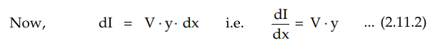
dV = I • z dx   i.e. dV / dx = I • z ... (2.11.1)

The current entering the element is I + di whereas the current leaving the element is I. The difference in the current di flows through the shunt admittance of the line. 

Differentiating equation (2.11.1) with respect to x,

Similarly we have after differentiating equation (2.11.2) with respect to x

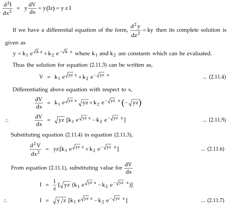
From equation (2.11.4) and (2.11.7) we get expression for V and I in the form of arbitrary constants k₁ and k₂. For finding the values of k₁and k₂, using the conditions which are given as,

At x = 0, V = V_R, I = I_R 

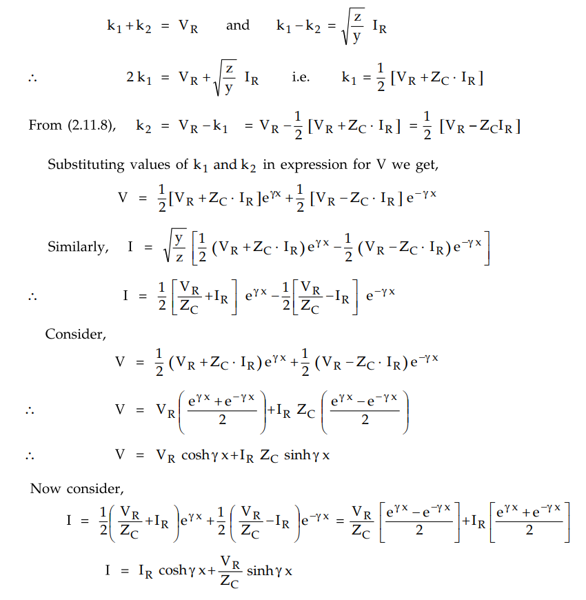
k₁ + k₂ = V_R  ... (2.11.8)

√ y/z [k₁ - k₂ ] = I_R  ... (2.11.9)

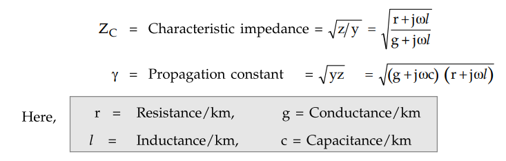
Two important constants of a transmission line which are complex quantities are as follows

Now from the equations (2.11.8) and (2.11.9)

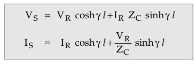
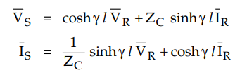
The sending end voltage V_S and current I_S are obtained by putting x = l in the expressions for V and I.

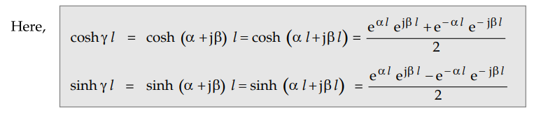
It is already been stated that Z_C and ɤ are complex quantities. The propagation constant ɤ can be expressed as,

ɤ = α + jβ

The real part of the propagation constant y is called the attenuation constant a and is measured in nepers per unit length. The imaginary part 3 is called the phase constant and is measured in radians per unit length.

 

1. Generalised Circuit Constants of a Long Transmission Line

By rigorous method the solution for sending end voltage obtained in case of long transmission line is given by,

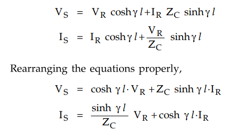
Comparing the above equations with the standard equations

 

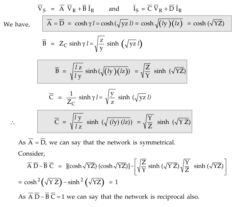
2. Evaluation of ABCD Constants

1) Convergent series method (Real angle method) : As ABCD constants are the hyperbolic functions of ɤl where ɤl = √ ZY is a complex quantity, ɤ may be written as complex quantity equal to α + j β where α and β are both real.

cosh ɤl = cosh (α + j β) l = cosh α l cosh j β l + sinh α l sinh j β l  

= cosh α l cos j β l  + jsinh α l sinh β l

Similarly, sinh ɤl = sinh (α + j β) l = sinh α l cosh j β l + cosh α l  sinh j β l

= sinh α l cos β l + jcosh α l sin α l

Using standard tables, sinh, cosh, sin and cos values can be obtained.

2) Convergent series method (Complex angle method) : To evaluate hyperbolic terms in the expression, we can make use of power series given by,

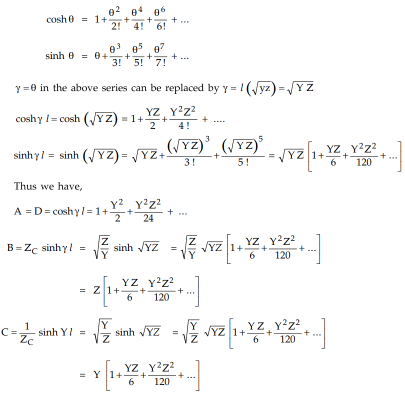
In this method, the series converges rapidly and sufficient accuracy can be obtained by considering first few terms. This method is preferred as compared to the method stated in (2.11.1) as it avoids use of tables and is comparatively less laborious.

The hyperbolic functions can also be evaluated by expressing them in terms of exponential such as

 

3. Evaluation of Voltage Regulation and Transmission Efficiency

By rigorous method of analysis of long transmission line, we have obtained the solution for sending end voltage and current as,

Comparing above equations with standard equations

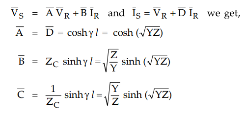
where Y = Total shunt admittance = y l, Z = Total series impedance = z l

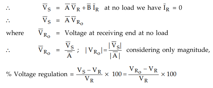
Voltage regulation is nothing but change in voltage at receiving end from no load to full load.

Thus following steps can be followed to obtain % voltage regulation.

1. Obtain A, B, C, D parameters for the long transmission line using given information.

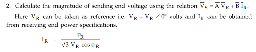
where cos ϕ _R is p.f. at receiving end.

3. Obtain the magnitude of no load voltage V_Ro at receiving end using the relation

| V_Ro | = | V_S | /  | A |

4. % Regulation of the line is then given as,

% Voltage regulation = V_Ro – V_R / V_R × 100

This procedure can in general be adopted to find the regulation of any type of transmission line.

To find the transmission efficiency, obtain the sending end current by using IS 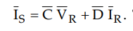. Then find the p.f. at sending end i.e. cos ϕ _S.

Power at sending end is then given as,

P_S = √ 3 V_S I_S cos ϕ _S

% Transmission efficiency =  Receiving end power / Sending end power × 100 = P_R / P_S × 100

The steps for computing % transmission efficiency can be summarized as

1. Obtain A, B, C and D parameters for the transmission line using given information.

2. Obtain sending end voltage and sending end current magnitudes by using following equations.

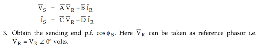
4. Compute the power at sending end

Sending end power, P_S = √ 3 V_S I_S cos ϕ _S

5. Power at receiving end P_R may be given. Thus % transmission efficiency is then given as,

Transmission efficiency (%) = P_R / P_S × 100

 

Example 2.11.1 A 3 phase transmission line 100 km long has the following constants.

Resistance / phase / km = 0.15 Ω , Reactance / phase / km = 0.20 Ω

Shunt admittance / phase / km = 1.5 × 10^-6 mho

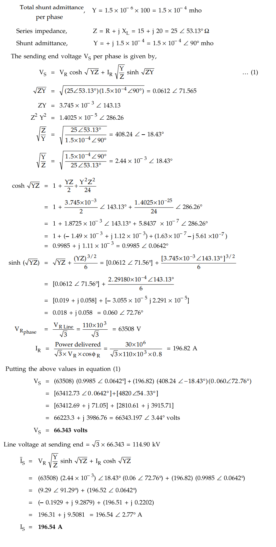
Calculate by rigorous method the sending end voltage and current when the line is delivering a load of 30 MW at 0.8 p.f. lagging. The receiving end voltage is kept constant at 110 kV.

Solution : Total resistance / phase, R = 0.15 × 100 - 15 Ω

Total reactance / phase, X_L = 0.20 × 100 = 20 Ω

 

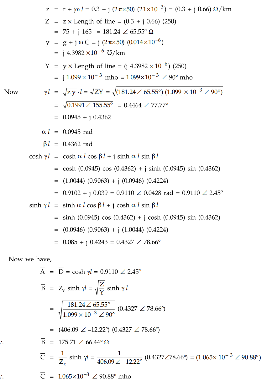
Example 2.11.2 Determine ABCD constants for a 3 phase 50 Hz transmission line 250 km long having the following distributed parameters

l = 2.1 × 10^-3 H/km , c = 0.014 × 10^-6 F/km, r = 0.30 Ω/km

Solution : We have,

 

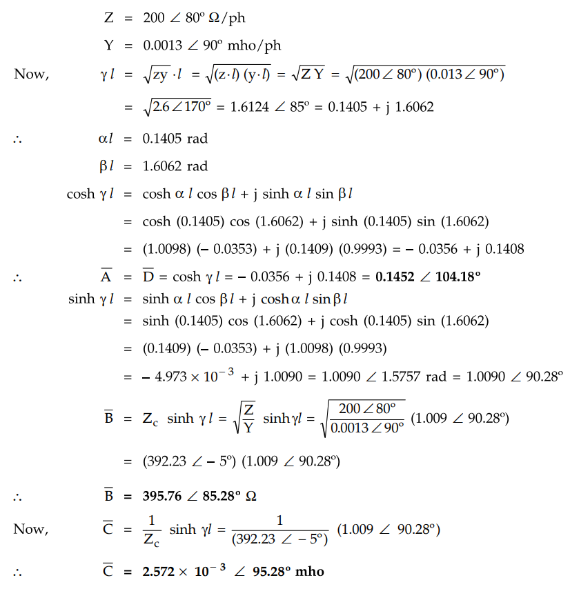
Example 2.11.3 A three-phase overhead long transmission line has total series impedance per phase (200 ∠ 80°) Ω and total shunt admittance of (0.0013 ∠ 90°) (mho/ph). The line deliver a load of 80 MW at 0.8 pf. lagging and 220 kV between lines. Determine A, B, C and D parameters.

Solution : We have,

Review Questions

1. State equation for long transmission line of VS and IS in term of Vr and Ir and line parameter per unit length. Derive this hyperbolic equation and discuss

i) Characteristics constant ii) Propagation constant

2. Derive expressions for the generalised A, B, C, D constants of a long transmission line by rigorous method cf analysis.

3. A3 phase transmission line 200 km long has the following constants Resistance/phase/km = 0.16 Ω, Reactance/phase/km = 0.25 Ω Shunt admittance/phase/km = 1.5 × 10^-6 mho

Calculate by rigorous method the sending end voltage and current when line is delivering load of 20 MW at 0.8 p.f. lagging. The receiving end voltage is kept at 110 kV.

[Ans : 116.67 kV, 131.1 A]

4. Determine ABCD constants for a 3 phase 50 Hz transmission line 200 km long having the following distributed parameters

5. Perform the analysis of long transmission lines using RIGOROUS method.

AU: Dec.-12, Marks 12

6. Explain the procedure for determining the transmission efficiency and voltage regulation of a long transmission line. AU May-05, Dec.-05, Marks 8 current relations in terms of receiving end

7. Derive for a long line the sending end voltage and voltage and current and the parameters of the line.

AU: Dec.-06, May-18, Marks 16