Sending End Power Circle Diagram

Sending End Power Circle Diagram

With the help of circle diagram at sending end we can get P_S,Q_S and power factor on complex plane.

The complex power at sending end is given by,

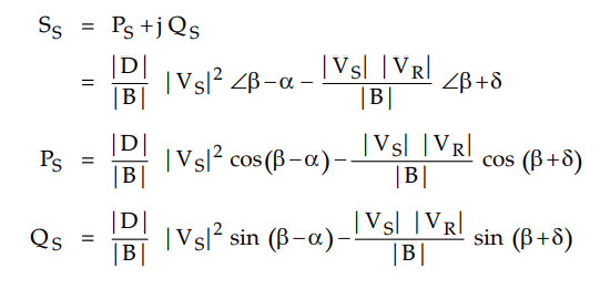
The sending end power circle diagram is shown in Fig. 2.17.1.

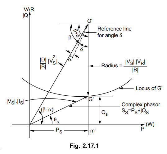
By the same method as for the receiving end circle diagram if V_R and V_S are kept constant then it can be proved that the point G' moves over a circle with centre O'. The co-ordinates of the centre are given as,

The radius of the sending end circle is given as,

Radius = | V_S | | V_R | / | B |

The radius is same as that obtained in case of receiving end circle diagram.

When sending end voltage is fixed, the position of centre O' is fixed and concentric circles are obtained with radii corresponding to different values of V R. However if |V_R | is fixed and it is required to draw sending end power circles for various values of  |V_S| then centre O' of sending end circle changes and lies along O'H'. This distance O'H' varies as | V_S|² and radii of the circles will also change as |V_S| keeps on changing.

If voltages |V_S | and |V_R | are fixed then P_S will be maximum when δ =180 – β

The sending end power circle diagram for a short transmission line is as shown in Fig. 2.17.2.

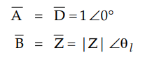
It is obtained by using the ABCD parameters for short line which are as follows.

Example 2.17.1 A 3 phase transmission line, 150 km long transmits a load of 80 MW at 0.8 p.f. lagging. The line voltage at the receiving end is 220 kV. The constants of the line A - D - 0.9785 ∠ 0.3°, B - 85.2 ∠ 77.47 °, C - 0.000503 ∠ 90.1 °

Draw receiving end and sending end circle diagrams for the transmission line and calculate

a) Sending end voltage, current, power factor, regulation and efficiency of the transmission line.

b) Load in kW at 0.8 p.f. lagging that could be carried at 8 % regulation.

c) Voltage drop if the load is 120 MW at the same power factor and the MVAR leading required for 120 MW load at 8 % regulation.

d) Rating and power factor of synchronous phase modifier connected in parallel with the load so that voltage transmitted at the sending end is same as that at the receiving end.

e) Maximum power that can be transmitted in case (d) Calculate the corresponding p.f.

Solution : The given values are

Let scales be selected as,

1 cm - 20 MW on horizontal axis

1 cm = 20 MVAR on vertical axis

So that we have 1 cm = 20 MVA

Steps for drawing the circle diagram

1. Locate the centre O with the co-ordinates as given above

2. Draw load line at an angle θ R = cos^-1 0.8 = 36.8° to the horizontal and cut

3. From the graph OP = 10.7 cm = 214 MVA

Steps for drawing sending end power circle diagram

1. Mark point O with co-ordinates obtained as above

2. Draw circle with

3. Draw OO₁ at angle of (β + δ)

The required answers are as follows :

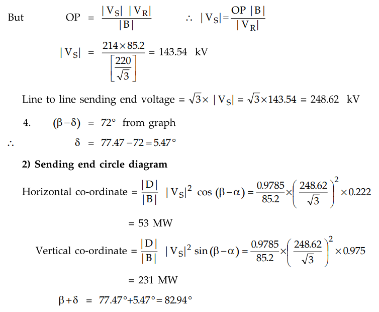
a) i) Sending end voltage = 248.62 kV (line value)

ii) Sending end current (I_S)

From the sending end circle diagram

Draw the new circle with the same centre but with radius of 10.2 cm. This circle cuts the load line at Px. Horizontal component of O-|P-| = 0.8 cm = 0.8x20 = 16 MW which is the load carried by the line per phase.

Total load carried at 8 % regulation = 3 × 16 = 48 MW

c) Power per phase = 120 / 3 = 40 MW

The new point P₂ can be marked on the load line corresponding to this load of 40 MW.

Drop per phase = 153-127 = 26 kV

The regulation required is 8% i.e. V_S = 1.08 V_R

For increased load, point P₂ must move vertically downward to cut circle (2) at M₂

Leading MVAR = P₂M₂ = 1.3 cm = 26 per phase

Total MVAR required = 26 × 3 = 78 MVAR

d) Here

Draw circle 3 with same centre but with radius 9.45 cm. P is the operating point if no leading MVAR is supplied by SPM. In this case the operating point M vertically downward on circle 3.

Leading MVAR = PM = 1.4 × 20 = 28 per phase

Total MVAR = 28 × 3 = 84 MVAR

e) Maximum power under these conditions can be found by drawing a horizontal line through O and cutting the circle at T'

Maximum power = TT' = 7.4 cm = 148 MW per phase = 444 MW for 3 phase

Power factor angle corresponding to this condition is 50.1°

p.f. = cos θ = cos 50.1° = 0.641 leading 

Example 2.17.2 The constants of a three phase line are A = 0.9Z2° and B = 140Z 70° ohms per phase. The line delivers 60 MVA at 132 kV and 0.8 pf lagging. Draw power circle diagrams and find (a) sending end voltage and power angle (b) the maximum power which the line can deliver with the above values of sending and receiving end voltage (c) the sending end power and power factor (d) line losses.

Solution : The given values are

Steps for drawing the sending end circle diagra, are as given below.

1) Locate the centre O with the co-ordinates as given above

2) Draw load line at an angle ϕ_R = cos10.8 = 36.86° to the horizontal and cut

3) From the graph OP = 13.9 cm = 55.6 MVA

The receiving end circle diagram is shown in the Fig. 2.17.4 (a)

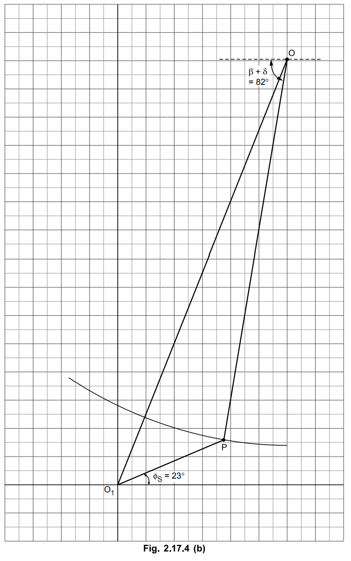
2) Sending end circle diagram

Steps for drawing the sending end circle diagra, are as given below.

1) Mark point O with co-ordinates given as above

2) Draw circle with radius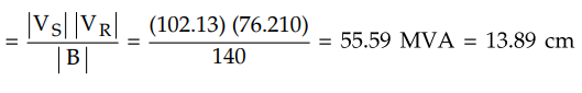 

3) Draw OO₁ at an angle of (β + δ) = 82°

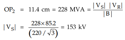
Sending end voltage (line value) = 176.89 kV

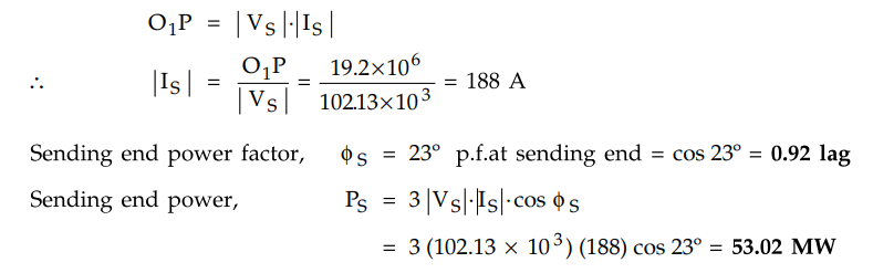
O₁P = 4.8 cm = 19.2 MVA (from circle diagram)

The sending end circle diagram is shown in the Fig. 2.17.4 (b)

Line Losses - Sending end power - Receiving end power = 53.02 - 48 = 5.02 MW

Maximum power that can be transferred

P_Rmax = N₁ P₁ = 10.4 cm = 10.4 × 4 = 41.6 MW per phase

For 3 phase max power transferred = 3 P_Rmax = 3 × 41.6 = 124.8 MW

Review Questions

1. Explain how sending end power circle diagram can be drawn.

2. A 275 kV three phase line has the following parameters

A = 0.93 ∠1.5°, B = 115 ∠77°

If the receiving end voltage is 275 kV calculate using circle diagram.

a) The sending end voltage required if a load of 250 MW at 0.85 lagging pf. is being delivered at the receiving end.

b) The maximum power that can be delivered if the sending end voltage is held at 295 kV.

c) The additional MVA that has to be provided at the receiving end when delivering 400 MVA at 0.8 lagging pf. the supply voltage being maintained at 295 kV.

[Ans.: 355.5 kV, 556 MW, 295 MVA]

3. A symmetrical 132 kV line delivers a load of 40 MW at 0.8 lagging of calculate with the help of circle diagram

a) The sending end voltage

b) The MVAR capacity of the synchronous condenser needed if the sending end voltage is increased to 180 kV.

c) The capacity of synchronous condenser needed at no load if the receiving end and sending end voltages are 132 kV respectively. Assume line constants are A = 0.9 ∠25°,

B = 100 ∠ 70°Ω, C = 0.0006 ∠ 88°.

[Ans.: 227.4 kV, 84 MVAR, 84 MVAR]

4. A 3 phase overhead line has per phase resistance and reactance of 6 Ω and 20 Ω respectively. The sending end voltage is 66 kV while the receiving end voltage is maintained at 66 kV by a synchronous phase modifier. Determine the kVAR of the modifier when the load at the receiving end is 75 MW at 0.8 pf. lagging also determine the maximum load that can be transmitted.

[Ans.: 96.95 MVAR, 148.67 MW]