Two - Way Classification

TWO-WAY CLASSIFICATION

In two-way classification of analysis of variance, we consider one classification along column-wise and the other along row-wise.

RBD [Randomized Block Design]

Let us consider an agricultural experiment using which we wish to test the effect of 'k' fertilising treatments on the yield of crops. We assume that we know some information about the soil fertility of the plots. Then, we divide the plots into 'h' blocks, according to the soil fertility each block containing 'k' blocks. Thus, the plots in each block will be of homogeneous fertility as far as possible within each block, the 'k' treatments are given to the 'k' plots in a perfectly random manner, such that each treatment occurs only once in any block. But the same k treatments are repeated from block to block. This design is called Randomized Block Design.

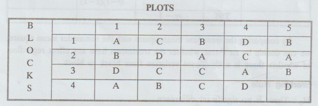
The scheme is most readily understood by visualising a field plan for an agricultural experiment, say for four treatments (A, B, C, D) in six blocks of four plots.

PLOTS

Merits and Demerits of Random Design

Merits

1. It has a simple layout.

2. The design controls the variability in the experimental units and gives the treatments equivalence to show their effects. nolistuotes sprismA

3. The analysis of the design is simple and straight forward as in the case of two-way classification of analysis of variance.

4. The analysis is possible, even in the case of missing observations.

Demerits

1. The design is not suitable for large number of treatments, since in this case the block size is large and hence homogeneity of units may not be possible.

2. Unequal number of replications for equal treatment is not possible.

 3. The shape of the experimental material should be rectangular.

4. It controls the variability in one direction only. aslo yew-owl al

5. The analysis of this decision is not as simple as a completely randomized design. Ingles old boximobas

The analysis of variance table for a randomized block design will, in general, have the following form.

 

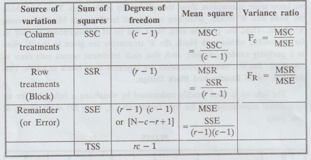
with the remainder mean square, we can decide by an F-test, whether the treatments have any effect regardless of whether there is a significant variation from block to block.

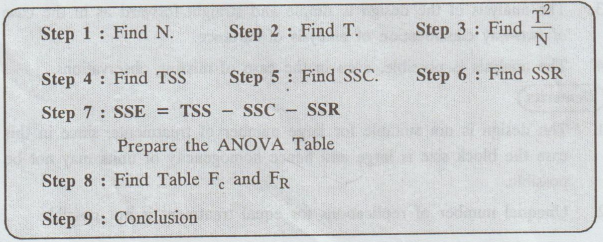
Working Rule

H₀ : There is no significant difference.

H₁ : There is a significant difference.

Test the hypothesis that variation between varieties and between blocks do not differ significantly from the variance due to random errors.

Arrange calculation of sum of squares.

 

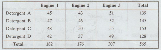
Example 2.3.1

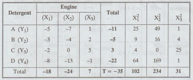
An experiment was designed to study the performance of 4 different detergents for cleaning fuel injectors. The following "cleanliness" readings were obtained with specially designed equipment for 12 tanks of gas distributed over 3 different models of engines:

Perform the ANOVA and test at 0.01 level of significance, whether there are differences in the detergents or in the engines.

[A.U. Model] [A.U. N/D. 2004] [A.U CBT A/M 2011] [A.U M/J 2007, N/D 2008] [A.U N/D 2015 R13]

Solution:

The above data are classified according to criteria (i) Detergent (ii) Engine.

In order to simplify calculations, we code the data by subtracting 50 from each figure.

H₀ : There is no significant difference between column means as well as

H₁ : There is significant difference between column means or the row means.

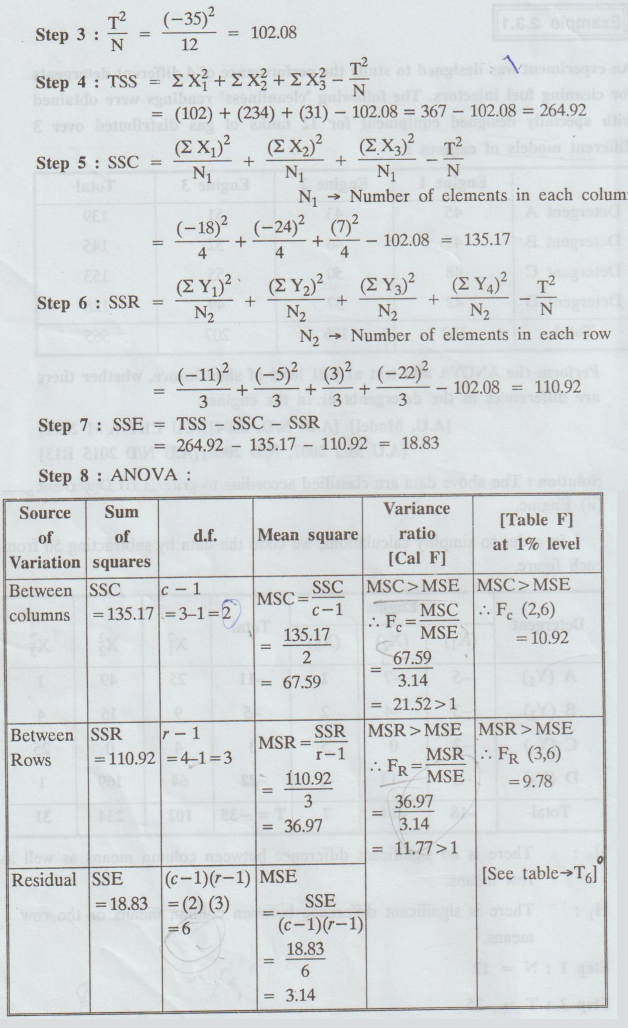
Step 1: N = 12

Step 2: T = -35

Step 9 : Conclusion .

(i) Cal Fe > table Fe, i.e., 21.52 > 10.92

So, we reject Ho for this case.

i.e., There are significant differences in the engines.

(ii) Cal F_R > table F_R, i.e., 11.77 > 9.78

So, we reject H₀ for this case.

i.e., There are significant differences in the detergents.

 

Example 2.3.2

Perform two-way ANOVA for the given below:

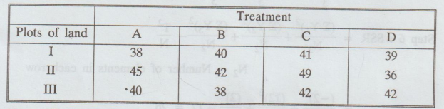
Use coding method, subtracting 40 from the given numbers.  [A.U. N/D 2005]

Solution:

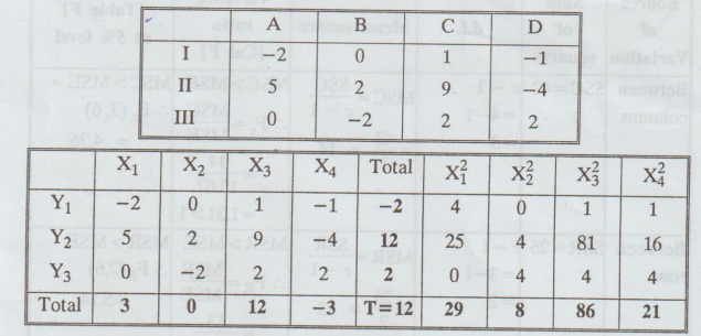
Subtract 40 from all the numbers. By doing so, F ratio is unaffected and reduces the numbers to smaller numbers.

H₀ : There is no significant difference between column means as well as

H_{1 :} There is significant difference between column means or the row means.

Step 1: N = 12

Step 2: T = 12

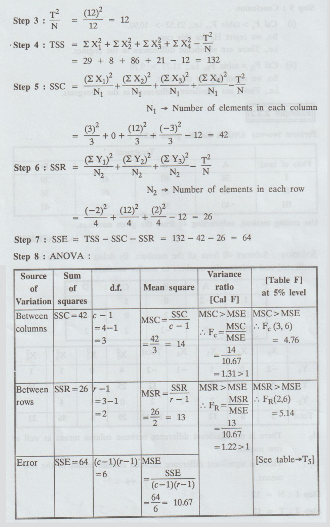
Step 9: Conclusion :

(i) Cal Fc < table Fe, i.e., 1.31 < 4.76

So, we accept Ho for this case.

i.e., There is no significant difference between treatments.

(ii) Cal F_R < table F_R, i.e., 1.22 < 5.14

So, we accept Ho for this case.

i.e., There is no significant difference between plots.

 

Example 2.3.3

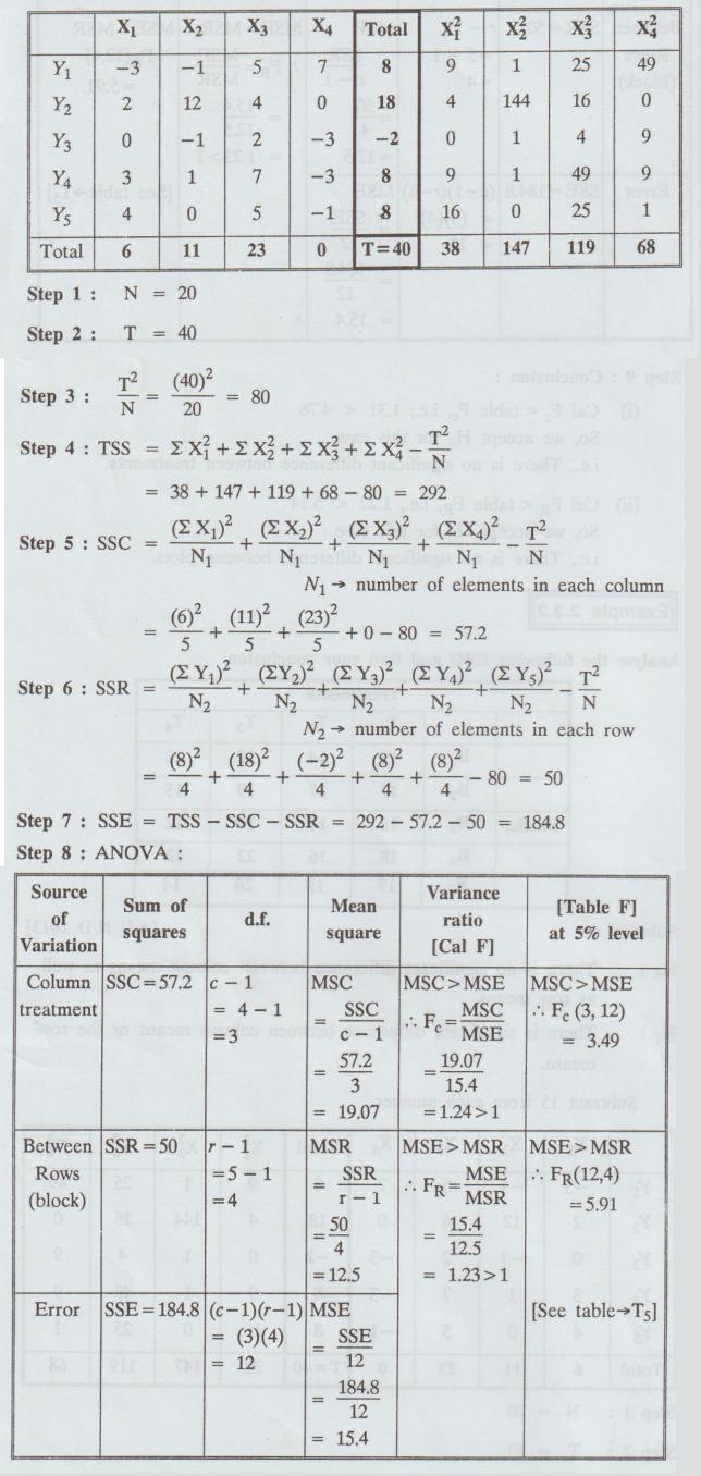
Analyse the following RBD and find your conclusion.

  

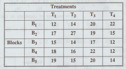
[A.U N/D 2013]

Solution :

H₀ : There is no significant difference between column means as well

H₁ : There is significant difference between column means or the row means.

Subtract 15 from each number.

Step 9 : Conclusion :

 (i) Cal Fe < Table Fe, i.e., 1.24 < 3.49.

So, we accept Ho for this case.

i.e., there is no significant difference between treatments.

(ii) Cal F_R < Table F_R, i.e., 1.23 < 5.91. So, we accept H₀ for this case.

i.e., there is no significant difference between blocks.

 

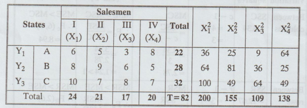
Example 2.3.4

The following table gives monthly sales (in thousand rupees) of a certain firm in the three states by its four salesmen.

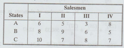
Setup the analysis of variance table and test whether there is any significant difference (i) between sales by the firm salesmen and (ii) between sales in the three states.

Solution :

H₀ : There is no significant difference between column means as well as

H₁ : There is significant difference between column means or the row means.

Step 1: N = 12

Step 2: T = 82

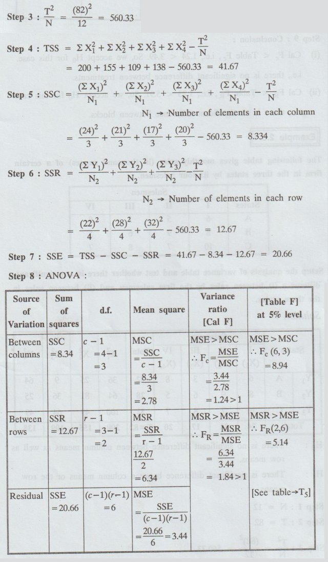
Step 9: Conclusion : 0

 (i) Cal Fe < Table Fe, i.e., 1.24 < 8.94. So, we accept H₀ for this case. i.e., there is no significant difference between salesmen.

(ii) Cal FR < Table FR, i.e., 1.84 < 5.14. So, we accept H₀ for this case.

i.e., there is no significant difference between states.

 

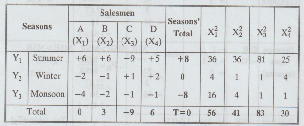
Example 2.3.5

A tea company appoints four salesmen A, B, C and D and observes their sales in three seasons summer, winter and monsoon. The figures (in lakhs) are given in the following table.

 (i) Do the salesmen significantly differ in performance ?

(ii) Is there significant difference between the seasons? 02M

 [A.U N/D 2012] [A.U M/J 2016 R13]

Solution: We code the data by subtracting 30 from each figure.

H₀ : There is no significant difference between column means as well as row means.

H₁ : There is significant difference between column means or the row means.

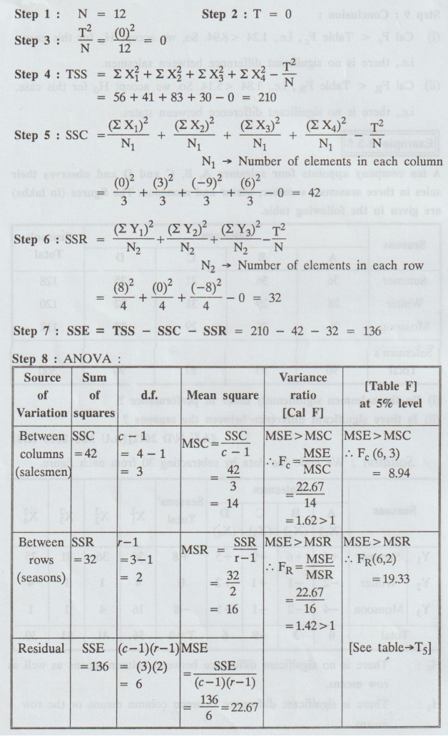
Step 9 Conclusion :

(i) Cal Fe < Table Fe, i.e., 1.62 < 8.94. So, we accept Ho for this case.

i.e., there is no significant difference between salesmen.

(ii) Cal FR < Table FR, i.e., 1.42 < 19.33. So, we accept Ho for this case.

i.e., there is no significant difference between seasons.

Thus, the test shows that the salesmen and the seasons are alike, so far as the sales are concerned.

 

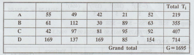
Example 2.3.6

A set of data involving "four tropical feed stuffs A, B, C, D" tried on 20 chicks is given below. All the twerty chicks are treated alike in all respects except the feeding treatments and each feeding treatment is given to 5 chicks. Analyze the data.

Weight gain of baby chicks fed on different feeding materials composed of tropical feed stuffs. [A.U A/M 2010] [A.U A/M 2017 R-13] [A.U N/D 2019 R-13]

Solution :

H₀ : There is no significant difference between column means as well as  row means.

H₁ : There is significant difference between column means or the row means.

Subtract 50 from each value

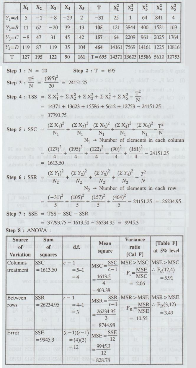
Step 9 : Conclusion:

(i) Cal Fe < Table Fe, i.e., 2.06 < 5.91. So, we accept H₀ for this case.

i.e., there is no significant difference between column means.

(ii) Cal FR > Table FR, i.e., 10.55 > 3.49. So, we reject H₀ for this case.

i.e., there are significant differences in row means.

 

Example 2.3.7

Three varieties A, B and C of a crop are tested in a randomised block design with four replications. The plot yield in pounds are as follows :

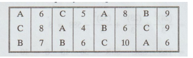
Analyse the experimental yield and state your conclusion.

[A.U N/D 2011] [A.U A/M 2019 R-13]

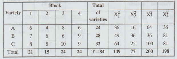
Solution :

Calculation of Correction factor

H₀ : There is no significant difference between column means as well as

H₁ :There is significant difference between column means or the row means.

Step 9 Conclusion :

(i) Cal Fe < Table Fe, i.e., 3.59 < 4.76. So, we accept Ho for this case.

i.e., there is no significant difference between blocks.

(ii) Cal F_R Table F_R, i.e., 2.4 < 5.14. So, we accept Ho for this case.

i.e., there is no significant difference between varieties.

 

Example 2.3.8

Four varieties A, B, C, D of a fertiliser are tested in a randomized block design with 4 replication. The plot yields in pounds are as follows : [A.U M/J 2014]

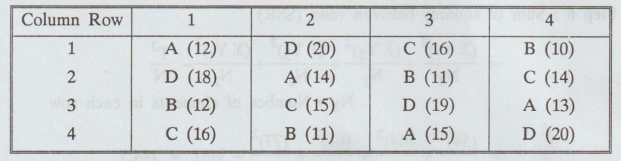
Analyse the experimental yield.

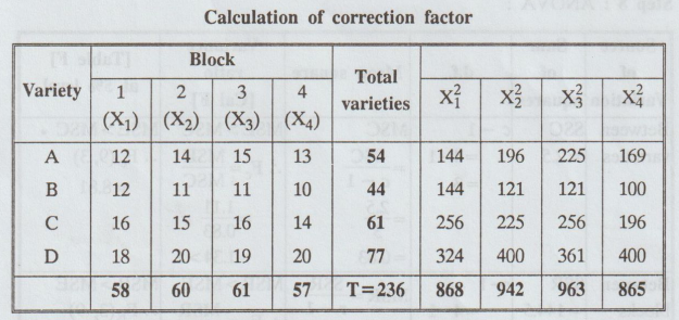
Solution:

Calculation of correction factor

H₀ : There is no significant difference between column means as well as row means.

H₁ : There is significant difference between column means or the row means.

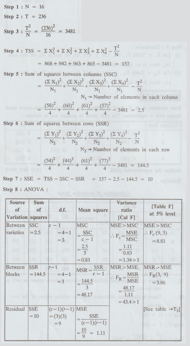
Step 9: Conclusion :

 (i) Cal Fe < Table Fe, i.e., 1.34 8.81. So, we accept Ho for this case.

i.e., there is no significant difference between blocks.boo

(ii) Cal FR > Table FR, i.e., 43.4 > 3.86. So, we reject Ho for this case.

i.e., there are significant differences in the varieties.

 

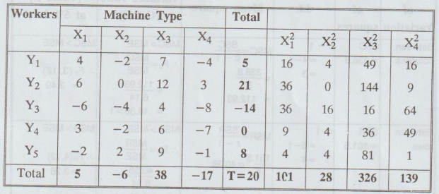
Example 2.3.9

The following data represent the number of units production per day turned out by different workers, using 4 different types of machines.

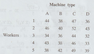
Test whether the five men differ with respect to mean productivity and test whether the mean productivity is the same for the four different machine types. [A.U. M/J 2006, N/D 2007, M/J 2013] [N/D 2010, A/M 2011]

Solution:

We subtract 40 from the given values we get the coded data is

H₀ : There is no significant difference between column means as well as row drown

H₁ : There is significant difference between column means or the row means.

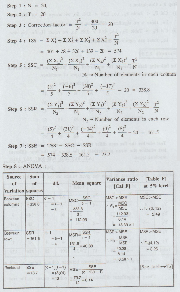
Step 9 Conclusion :

 (i) Cal Fe > Table Fe, i.e., 18.39 > 3.49. So, we reject Ho for this case.

i.e., there are significant differences in the machines.

(ii) Cal FR > Table FR, i.e., 6.58 > 3.26. So, we reject Ho for this case.

i.e., there are significant differences in the workers.

Hence, the 5 workers differ significantly and the 4 machine types also differ significantly with respect to mean productivity.

 

Example 2.3.10

The table shows the yield of paddy in arbitrary units obtained from four different varieties planted in five blocks where each block is divided into four plots. Test at 5% level whether the yields vary significantly with (i) soil differences (ii) differences in the type of paddy.

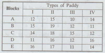
 [A.U N/D 2017 (R17)] [A.U N/D 2019 (R17)]

Solution :

H₀ : There is no significant difference between column means as well as row means.

H₁ : There is significant difference between column means or the row means.

EB SS

Subtract 14 from each number.

Step 9: Conclusion :

 (i) Cal Fe > Table Fe, i.e., 5.82 > 3.49. So, we reject H₀ for this case.

i.e., there are significant differences between types of paddy.

(ii) Cal FR < Table FR, i.e., 1.55 < 5.91. So, we accept H₀ for this case.

i.e., there is no significant difference in the blocks.

 

Example 2.3.11

Table below shows the seeds of 4 different types of corns planted in 3 blocks. Test at 0.05 level of significance whether the yields in kilograms per unit area vary significantly with different types of corns.

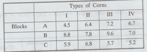
[A.U A/M 2019 R-17] [A.U N/D 2020 R-17]

Solution :

H₀ : There is no significant difference between blocks and types of corns.

H₁ : There is significant difference between blocks and types of corns.

Subtract 6.8 from all the numbers

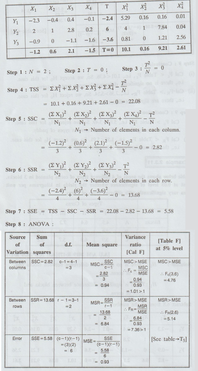
Step 9: Conclusion :

(i) Cal Fe < Table Fe, i.e., 1.01 <4.76. So, we accept H₀ for this case.

i.e., there is no significant difference between types of corns.

(ii) Cal-F_R.> Table F_R i.e., 7.36 > 5.14. So, we reject Ho for this case.

i.e., there are significant differences in blocks. 0+ 1.01