Analysis of Pulse Mode Asynchronous Circuits

Analysis of Pulse Mode Asynchronous Circuits

• In the analysis of pulse mode asynchronous sequential circuits, circuits respond immediately to pulse on their inputs, rather than waiting for clock signal, as in synchronous sequential circuits. The pulse mode circuits assume that pulses do not occur simultaneously on two or more input lines, means that a circuit with n input lines has only n + 1 input conditions, rather than 2ⁿ, as is the case for synchronous circuits. They also assume that a state transition can occur only if an input pulse occurs. Hence, the memory elements of the circuit respond only when an input pulse arrives. Keeping these assumptions in mind, let us examine the behaviour of the pulsed asynchronous circuit in the example 7.3.1.

Examples for Understanding

Ex. 7.3.1 Analyse the given pulsed asynchronous sequential circuit

Sol. :

Step 1 : Determine the circuit excitation and output equations.

For given circuit excitation and output equations are :

Step 2 : Determine the next state equation of state variable.

The characteristic equation for SR flip-flop is

Using the characteristic equation and excitation equations we have the state variable next state equation is as follows :

Step 3 : Construct the state variable transition table.

From next state and output equations we can construct the state variable transition table indicating state variables, input variables, next state values and the output value.

Step 4: Derive the flow table and state diagram.

From the state variable transition table we can derive the flow table and from flow table we can derive the state diagram as shown in the Fig. 7.3.3. The flow diagram can be constructed by replacing next state and state variable values by actual states S1 = 0 and S₁ = 1.

Step 5 : Draw the timing diagram.

The Fig. 7.3.4 shows the timing diagram for the pulse mode circuit shown in the Fig. 7.3.1. As shown in the timing diagram, the inputs are the pulses and they occur one at a time.

Ex. 7.3.2 Consider the asynchronous sequential circuit which is driven by the pulses, as shown in the Fig. 7.3.5. Analyze the circuit.

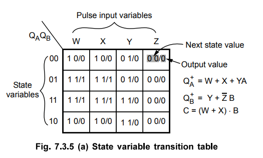
Sol. : The circuit has two NAND gate latches that generate the state variables, A and B. The circuit has four input variables W, X, Y and Z and one output variable C.

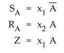
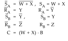
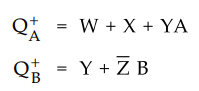
Step 1 : Determine the circuit excitation and output equations.

From the given sequential circuit we can have excitation and output equations as follows :

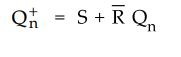
Step 2 : Determine next state equations for state variables.

The characteristic equation for SR flip-flop is

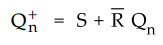
Using the characteristic equation and excitation equations we have the state variable next-state equations as follows

Step 3 : Construct the state variable transition table. From these next state and output equations we can construct the state variable transition table indicating state variables, input variables, next state values and the output-state.

Step 4: Derive the flow table and state diagram.

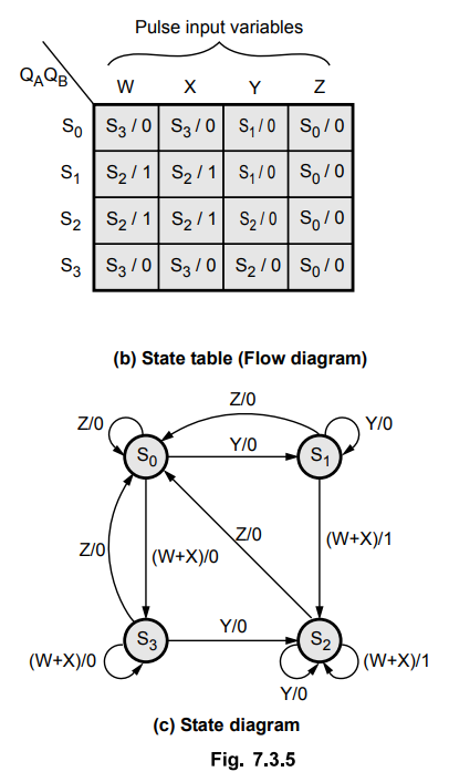
From the state variable transition table we can derive the flow table and from flow table we can derive the state diagram as shown in the Fig. 7.3.5 (b) and (c). The flow diagram can be constructed by replacing next state and state variable values by actual states

(S₀ = 00, S₁ = 01, S₂ = 11 and S₃ = 10).

Ex. 7.3.3 Consider the asynchronous sequential circuit driven by the pulses shown in Fig. 7.3.6. Analyze the circuit and draw the timing diagram.

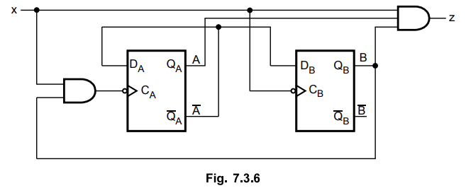
Sol. :

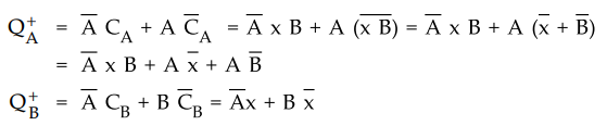
Step 1 : Determine the circuit excitation and output equations.

From the given sequential circuit we can have excitation and output equations as follows :

Step 2 : Determine the next state equations for state variables.

The characteristic equation for D flip-flop is

Q⁺_n = D and considering clock input it is given as

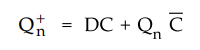
Using the characteristic equation and excitation equations we have the state variable next state equations as follows :

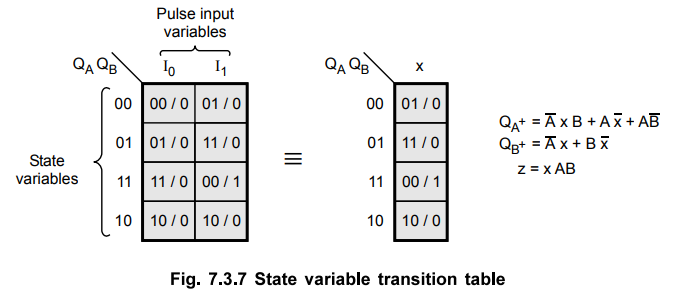
Step 3 : Construct the state variable transition table.

From these next state and output equations we can construct the state variable transition table indicating state variables, input variables, next state values and the output state.

A state variable transition table may be compiled for this circuit if we define the following.

Input: I₀ = No pulse on x

I₁ = Pulse on x 

States : AB : 00, 01, 10, 11

Output: z = 0, z = 1

Step 4: Derive the flow table and state diagram.

From the state variable transition table we can derive the flow table and from flow table we can derive the state diagram as shown in the Fig. 7.3.8. The flow diagram can be constructed by replacing next state and state variable values by actual states

(S₀ = 00, S₁ = 01, S₂ = 11 and S₃ = 10).

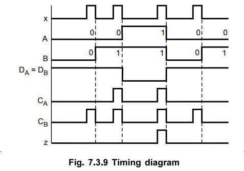
Step 5 : Draw the timing diagram.

The Fig. 7.3.9 shows the timing diagram for the given circuit.

Example for Practice

Ex. 7.3.4 Analyze the pulse-mode circuit shown in Fig. 7.3.10. Determine flow table and state diagram.

Review Question

1. Describe the procedure of analysis of pulse mode asynchronous circuit with the help of example.