Large sample test (Normal distribution) for difference of means

Large sample test (Normal distribution) for difference of means :

Consider two different normal populations with mean μ₁ and M₂ and S.D σ₁ and σ₂ respectively. Let a sample of size n₁ be drawn from the first population and an independent sample of size n₂ be drawn from the second population. Let  be the mean of the first sample from the first population and  be the mean of the second sample from the second population. If the sample sizes are large, we know  is a normal variate with mean μ₁ and

Variance σ²₁ / n₁ is an independent normal variate with mean µ₂ and variance

σ²₂ / n2

Therefore, the difference  of the two independent normal variates  and  is also independent normal variate. Hence the standard normal (x1-x2)-E (x1-X2)

Now, set the hypothesis H₀ : µ₁ = µ₂ (there is no significant difference between the sample means).

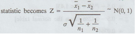
Thus, under H₀, the test statistic becomes Z =  which can be tested at any level of significance.

Note 1. If the samples have been drawn from the 2 distinct populations with common s.d σ, then under the null hypothesis the above test

which can be tested at any level of significance.

Note 2. If the common s.d o is not known, then its estimate based on the sample variances s²₁ and s²₂ can be obtained as 

In this case the test statistic becomes

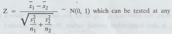
Note 3.If σ²₁ ≠ σ²₂ and σ₁ and σ₂ are not known, then they can be estimated from the sample variances as σ²₁ ~ s²₁ and σ²₂ ~ s²₂ In this case the test statistic becomes

required level of significance.

Working Procedure :

Concerning two means, with known variances σ₁ and σ₂.

For the large samples (n₁, n₂ > 30) to test the hypothesis for difference of means, whether μ₁-μ₂ = δ constant = 0 or not.

1. Null hypothesis H₀ : μ₁ = μ₂

(r)ds.r slomsx3

2. Alternative hypothesis H₁: μ₁ ≠ μ₂ (or)

H₁ μ₁ > μ₂ (or) H₁: μ < μ₂

The application of one-tailed or two-tailed test depends upon the nature of the alternate hypothesis.

The choice of the appropriate alternative hypothesis depends on the situation and the nature of the problem concerned.

For example:

Suppose, there are two brands of tyres, one manufactured by standard process with mean life μ1 and the other manufactured by new technique with mean life μ₂

Two-tailed test : If our test is whether the tyres differ significantly, then H₀ μ₁ = μ₂ and H₁: μ₁ ≠ μ₂

One-tailed test (left) : If our test is the tyres produced by the new process have a higher average life, then H₀ : μ₁ = μ₂ and H₁ = μ₁ < μ₂

One-tailed test (right): If your test is the tyres produced by the new process is inferior, then H₀ : μ₁ = μ₂ and H₁ : μ₁ > μ₂

3. Level of significance: ɑ

4. Critical region:

(a) μ₁ ≠ μ₂ [two-tailed test]

(b) μ₁ < μ₂ [one-tailed test (left)]

(c) μ₁ > μ₂ [one-tailed test (right)] 10

5. The test statistic:

6. Conclusion :

(a) If -Z_ɑ/2 < Z < Z _ɑ/2, then we accept Ho; otherwise, we reject Ho

(b) If Z < Z_ɑ, then we accept H₀; otherwise, we reject H₀.

(c) If - Z_ɑ < Z, then we accept H₀; otherwise, we reject H₀

 

Example 1.2b(1)

Examine whether the difference in the variability in yields is significant at 5% level of signification for the following:

 

Example 1.2b(2)

The means of two large samples of 1000 and 2000 members are 67.5 inches and 68.0 inches respectively. Can the samples be regarded as drawn from the same population of standard deviation 2.5 inches? [A.U M/J 2012]

Solution:

Given:

 

Example 1.2b (3)

Random samples drawn from two countries give the following data relating to the heights of adult males. Is the difference between standard deviation significant? [A.U M/J 2013]

6. Conclusion:

Here, Cal Z < table Z

i.e., 1.56 < 1.96

So, we accept Ho at 5% level of significance.

 

Example 1.2b(4)

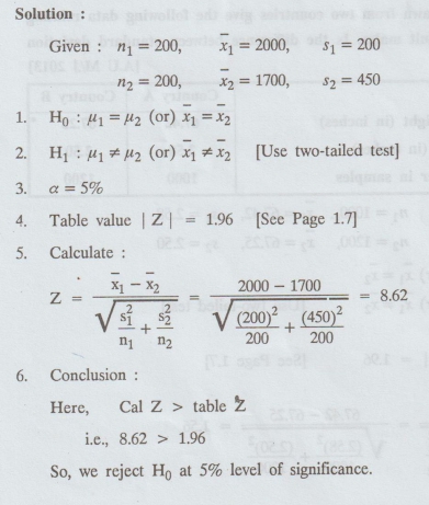
The sales manager of a large company conducted a sample survey in two places A and B taking 200 samples in each case. The results were in the following table. Test whether the average sales is the same in the two areas at 5% level. [A.U. N/D 2013]

Solution :

Example 1.2b(5)

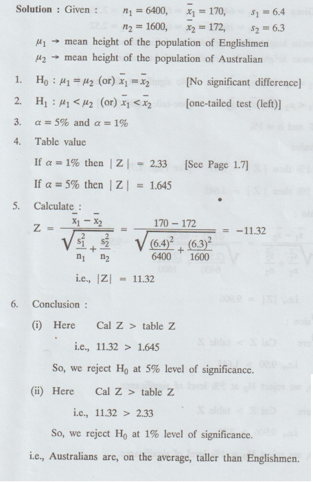
A simple sample of heights of 6,400 Englishmen has a mean of 170 inches and a standard deviation of 6.4 inches, while a simple sample of heights of 1600 Australians has a mean of 172 inches and a standard deviation of 6.3 inches. Do the data indicate that Australians are on the average taller than Englishmen ?MU [A.U. N/D 2007]

Solution:

 

Example 1.2b (6)

A sample of heights of 6400 Englishmen has a mean of 67.85 inches and a S.D of 2.56 inches, while a sample of heights of 1600 Australians has a mean of 68.55 inches and a S.D. of 2.52 inches. Do the data indicate that Australians are on the average taller than Englishmen?ted) stealbai atch sd of adoni [TOOS QUA] [A.U. N/D 2007] [A.U N/D 2019 R-17]

Solution:

 

Example 1.2b(7)

In a random sample of size 500, the mean is found to be 20. In another independent sample of size 400, the mean is 15. Could the samples have been drawn from the sample population with S.D 4?

Solution :

Example 1.2b(8)

The average marks scored by 32 boys is 72 with a S.D. of 8, while that for 36 girls is 70 with a S.D. of 6. Test at 1% level of significance whether the boys perform better than girls.dolla

Solution:

 

Example 1.2b(9)

The mean height of 50 male students who showed above average participation in college athletics was 68.2 inches with a standard deviation of 2.5 inches; while 50 male students who showed no interest in such participation had a mean height of 67.5 inches with a standard deviation of 2.8 inches. (a) Test the hypothesis that male students who participate in college athletics are taller than other male students. (b) By how much should the sample size of each of the two groups be increased in order that the observed difference of 0.7 inches in the mean heights be significant at the 5% level of significance. [A.U N/D 2016 (R13)]

Solution:

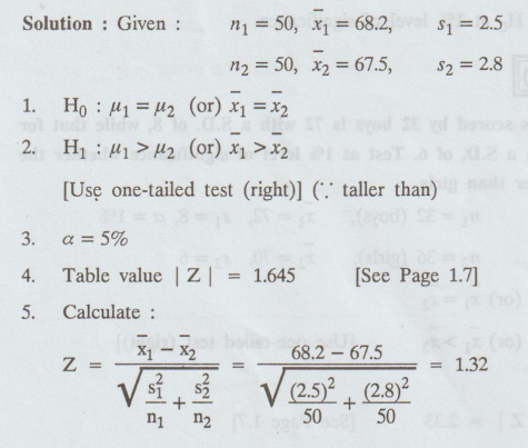
6. Conclusion :

Here Cal Z < table Z

i.e., 1.32 < 1.645

So, we accept H₀ at 5% level of significance.

We conclude that the college athletes are not taller than other male students.

(b) The difference between the mean heights of two groups, each of size

n will be significant at 5% level of significance if Z ≥ 1.645.

Hence, the sample size of the two groups should be increased by atleast 78 50 = 28, in order that the difference between the mean heights of the two groups is significant.

 

Example 1.2b(10)

Two samples drawn from two different populations gave the following results:

Test the hypothesis, at 5% level of significance, that the difference of the means of the population is 35.

Solution:

6. Conclusion :

Here Cal Z < table Z

i.e., 1.9 < 1.96

So, we accept H₀ at 5% level of significance.

 

Example 1.2b(11)

A sample of 100 bulbs of brand A gave a mean lifetime of 1200 hours with a S.D. of 70 hours, while another sample of 120 bulbs of brand B gave a mean lifetime of 1150 hours with a S.D. of 85 hours. Can we conclude that brand A bulbs are superior to brand B bulbs ?

Solution:

6. Conclusion:

Here  Cal Z >  table Z

i.e., 4.79 > 2.33

So, we reject Ho at 1% level of significance.

 

Example 1.2b(12)

The sales manager of a large company conducted a sample survey in states A and B taking 400 samples in each case. The results were in the following table. Test whether the average sales is same in the 2 states at 1% level. [1201 bolist-[A.U. M/J 2013] [A.U A/M 2017 R-13]

Solution:

6. Conclusion:

Here   Cal Z > table Z

i.e., 8.82 > 2.58

So, we reject H₀ at 1% level of significance.

 

Example 1.2b(13)

A mathematics test was given to 50 girls and 75 boys. The girls made an average grade of 76 with a SD of 6, while boys made an average grade of 82 with a SD of 2. Test whether there is any significant difference between the performance of boys and girls. [A.U N/D 2012 R-08, A.U M/J 2016 R-13]

Solution :

6. Conclusion:

Here, Cal Z > Table Z

i.e., 6.82 > 1.96

So, we reject H₀ at 5% level of significance.

 

Example 1.2b(14)

Test the significance of the difference between the means of the samples, drawn from two normal populations with the same S.D. from the following data :

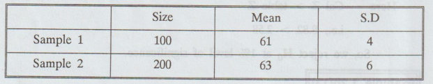
Solution:

6. Conclusion :

Here, Cal Z > table Z

i.e., 3.43 > 1.96

So, we reject Ho at 5% level of significance.

i.e., The two normal populations, from which the samples are drawn, may not be same mean, though may have the same s.d.

 

EXERCISE 1.2.(a) and 1.2(b)

Tests based on Normal distributions for means and difference of means.

1. A sample of 900 items has mean 3.4 and standard deviation 2.61. Can the sample be regarded as drawn from a population with mean 3.25 at 5% level of significance ?

Ans. |z| = 2.67

2. An automatic machine fills tea in sealed tins with nan weight of tea 1 kg and S.D 1 gm. A random sample of 50 tins was examined and it was found that their mean weight was 999.50 gms. Is the machine working plovige properly?

Ans. |z| = 3.54

3. A sample of 1000 students from Madras University was taken and their average weight was found to be 112 pounds with a S.D of 20 pounds. Could the mean weight of the student in the population be 120 pounds.

Ans. |z | = 12.66

4. The average income of persons was Rs. 210 and with Rs. 10 for S.D. in a sample of 100 people of city. For another sample of 150 people the average income was Rs. 220 and S.D of Rs. 12. Test whether there is any significant difference between the average income of the locality.

5. In a survey of buying habits, 400 women shoppers are chosen at random in super market 'A' located in a certain section of the city. Their average weekly food expenditure is Rs. 250 with a S.D of Rs. 40. For 400 women shoppers chosen at random in super market 'B' in another section of the city, the average weekly food expenditure is Rs. 220 with a S.D. of Rs. 55. Test at 1% level of significance whether the average weekly food expenditure of the two populations of shoppers are equal.

6. The average hourly wage of a sample of 150 workers in a plant 'A' was Rs. 2.56 with S.D. of Rs. 1.08; The average wage of a sample of 200 workers in plant 'B' was Rs. 2.87 with a S.D of Rs. 1.28. Can an applicant safely assume that the the hourly wages paid by plant 'B' are higher than those paid by plant 'A'?

7. The mean produce of wheat of a sample of 100 fields comes to 200 kg per acre and another sample of 150 fields gives the mean of 220 kg. Assuming the S.D of the yield at 11kgs for the universe, test if there is a significant difference between the means of the samples.

8. The means of two large samples of sizes 2000 and 1000 are 68.0 and 67.5 gms respectively. Can the sample be regarded as drawn from the same population of S.D 2.25 gms.

9. In a certain factory there are two independent processes of manufacturing the same item. The average weight in a sample of 250 items produced from one process is found to be 120 ozs with a S.D of 12 ozs. While the corresponding figures in a sample of 400 items from the other process are 124 and 14. Find the S.E of difference between the two sample means. Is this difference significant? Also find the 99% confidence limits for the difference in the average weights of items produced by the two processes respectively.