Large sample test for Single proportion

Large sample test for Single proportion

I. Test for a Single proportion

If X is the number of successes in n independent trials with constant probability P of success for each trial.

E(X) = nP and V(X)  = nPQ

where Q = 1 P, is the probability of failure.

It has been proved that for large n, the binomial distribution tends to normal distribution. Hence for large

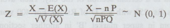
and we can apply the normal test.

 

Example 1.2.c(1)

In a sample of 1,000 people in Maharashtra, 540 are rice eaters and the rest are wheat eatrs. Can we assume that both rice and wheat are equally popular in this state at 1% level of significance.

Solution:

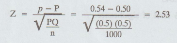
Given: n = 1,000, X = 540, p = X / n = 540 / 1000 = 0.5

P = Population proportion of rice eaters in Maharastra = 1/2 = 0.5

Q = 1 - P = 1- 1/ 2 = 1/2  = 0.5

1. H₀ P = 0.5 [Both rice and wheat eaters are equally popular in the state]

2. H₁: P  ≠ 0.5

3. ɑ = 0.01

4. Table value |Z| = 2.58

5. Calculate :

6. Conclusion :

Here, Cal Z < table Z

i.e., 2.53 < 2.58

So, we accept H₀ at 1% level of significance.

We may conclude that rice and wheat eaters are equally popular in Maharashtra state.

 

Example 1.2.c(2)

Twenty people were attacked by a disease and only 18 survived. Will you reject the hypothesis that the survival rate, if attacked by this disease, is 85% in favour of the hypothesis that it is more, at 5% level. (use large sample test) [A.U. N/D 2013]

Solution:

Given: n = 20

Mal slqooq 000, I to

X = number of persons who survived after attack by a disease = 18

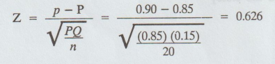
p = X / 20 = 0.90

P = 0.85

Q = 1 - 0.85 = 0.15

1. H₀ : P = 0.85 [no significant difference]

2. H₁ : P > 0.85 [One tail test]

3. ɑ = 0.05

4. Table value |z| = 0.626

5. Calculate :

6. Conclusion :

Here, Cal Z < table Z

i.e., 0.626 < 1.645

So, we accept Ho at 5% level of significance.

 

Example 1.2.c(3)

A manufacturer claimed that at least 95% of the equipment which he supplied to a factory conformed to specifications. An examination of a sample of 200 pieces of equipments revealed that 18 were faulty. Test his claim at a significance level of (i) 5% (ii) 1%.

Solution:

Given n = 200

X = Number of pieces conforming to specifications in the samples

 = 200 - 18 = 182

p = Sample proportion conforming to specifications

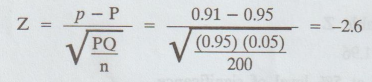
P = 0.95, Q = 1 P = 1 0.95 = 0.05

1. H₀ : P = 0.95 [The proportion of pieces conforming to specification in the population is 95%]

2. H₁ P < 0.95 [at least 95% conformed to the specification]

3. (i) ɑ = 0.05, (ii) ɑ =  0.01

4. Table value

(i) |Z| > 1.645 at 5% level.

(ii) |Z| >  2.33 at 1% level.

5. Calculate :

6. Conclusion:

(i) Here, Cal Z > table Z

i.e., 2.6 > 1.645

So, we reject Ho at 5% level of significance.

(ii) Here, Cal Z > table Z

i.e., 2.6 > 2.33

So, we reject Ho at 1% level of significance.

 

Example 1.2.c(4)

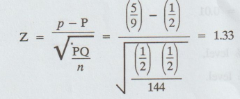
A coin is tossed 144 times and a person gets 80 heads. Can we say that the coin is unbiased one ?

Solution:

Given n =144

P = probability of getting a head in a toss = 1 / 2

Q = 1 - P = 1 – 1 / 2 = 1 / 2

X = number of successes

= number of getting heads = 80.

P = X / n = 80 / 144 = 5 / 9

1. H₀  = [the coin is unbiased]

2. H₁ : the coin is biased

3. ɑ = 0.05

4. Table value |Z | = 1.96

5. Calculate :

6. Conclusion :

Here, Cal Z < table Z

i.e., 1.33 < 1.96

So, we accept H₀ at 5% level of significance.

Hence the coin is unbiased.

 

Example 1.2.c(5)

In a big city 325 men out of 600 men were found to be smokers. Does this information support the conclusion that the majority of men in this city are smokers.

Solution:

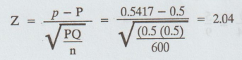
Given: n = 600, P = 325 / 600 = 0.5417

P = Population proportion of smokers in the city = 0.5

Q = 1- P = 10.5 = 0.50

1. H₀ : p = 0.5

2. H₀ :  p > 0.5

3. ɑ = 1% and 5%

4. Tabulate | Z |= 2.33, 1% level

| Z |= 1.645, 5% level

5. Calculate

6. Conclusion :

(i) Here, Cal Z < table Z

i.e., 2.04 < 2.33

So, we accept Ho at 1% level of significance.

(ii) Here, Cal Z > table Z

i.e., 2.04 > 1.645

So, we reject H₀ at 5% level of significance.

Note: We cannot come to solid conclusion from this random sample data. We may try for some other sample data for deciding whether majority of men in that city are smokers.

 

Example 1.2.c(6)

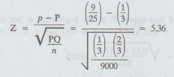
A dice is thrown 9,000 times and a throw of 3 or 4 is observed 3,240 times. Show that the dice cannot be regarded as an unbiased one and find the limits between which the probability of a throw of 3 or 4 lies.

Solution:

Given: n = 9,000

X = Number of successes

= Probability of success

= Probability of getting a 3 or 4 = 1/ 6 + 1/6 = 1/3

Q = 1 – 1/3 = 2/3

P = X / n = 3240 / 9000 = 9/25

1. H₀ : P = 1/3 [unbiased]

2. H₁: P ≠ 1/3

3. ɑ not given.

4. Table value |Z | = 3 for both the level of significance.

5. Calculate :

6. Conclusion :

Since |Z| = 5.36 > 3 so we reject H₀.

We conclude that the dice is almost certainly biased.

Since dice is not unbiased, P ≠ 1/3

The probable limits for 'P' are given by

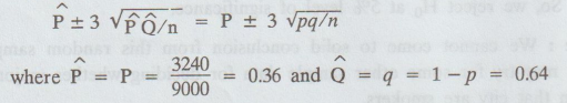
Hence the probable limits for the population proportion of successes may be taken by

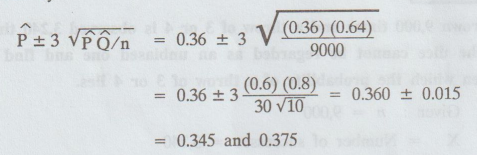
Hence the probability of getting 3 or 4 almost certainly lies between 0.345 and 0.375.

 

Example 1.2.c(7)

A random sample of 500 apples was taken from a large consignment of apples and 65 were found to be bad. Find the S.E of the population of bad ones in a sample of this size. Hence deduce that the percentage of bad apples in the consignment almost certainly lies between 8.5 and 17.5.

Solution:

Given n = 500.

Let X = number of bad apples in the sample 65.

p = proportion of bad apples in the sample = 65 / 500 =  0.13.

Hence q = 0.87

Here the proportion of bad apples P in the population is not known.

Hence we can take P = p 0.13 and Q = q = 0.87 and n = N = 500.

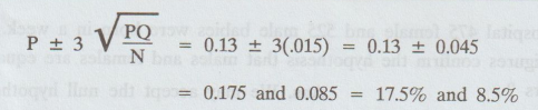
S.E of proportion √PQ / N =  √0.13 × 0.87/ 5000 = 0.015

Limits for proportions of bad apples in the population is

 

EXERCISE 1.2(c)_______

1. A person threw 10 dice 500 times and obtained 2560 times 4, 5 or 6. smo Can this be attributed to fluctuations in sampling ?

Ans. z 1.697

2. The difference could be attributed to fluctuations in sampling. While throwing 5 dice 30 times a person obtained success 23 times (securing a 6 was considered a success). Can we consider the difference between the observed and the expected results as being significantly different ?

Ans. z 0.438

The difference between the sample proportion and the population proportion is not significant.

3. In a sample of 500 people in Kerala 280 are tea drinkers and the rest are coffee drinkers. Can we assume that both coffee and tea are equally popular in the state at 5% level of significance ?

Ans. z = 2.68

Therefore coffee and tea are not equally popular in that state.

4. In a sample of 600 parts manufactured by a factory, the number of defective parts was found to be 45. The company however claimed that only 5% of their product is defective. Is the claim tenable?

Ans. z = 2.8

5. Sky packets managing director says with 95% confidence that there has been a significant improvement in deliveries based on a sample of 81 deliveries out of which 6 were late. If in general 10% of deliveries were late in the past, should Managing Director's statement be accepted?

Ans. z = 0.78

6. In a certain city 380 men out of 800 are found to be smokers. Discuss whether this information supports the view that majority of men in this city are non-smokers.

Ans. z = 1.414

We cannot conclude that majority are non-smokers.

7. A coin is tossed 400 times and it turns up head 216 times. Discuss whether the coin is an unbiased one. [A.U N/D 2011]

Ans. The coin is unbiased

8. A person throws 10 dice 500 times and obtain 2560 times 4, 5 or 6. Can this be attributed to fluctuations in sampling. Explain.

9. In a hospital 475 female and 525 male babies were born in a week. Do these figures confirm the hypothesis that males and females are equal in numbers ?8 bas

Ans. We may accept the null hypothesis.

10. Balls are drawn from a bag containing same number of black and white balls, each ball being returned before drawing another. In 2250 drawings, 1018 black and 1232 white balls have been drawn. Do you suspect some rea bias on the part of the drawer.

Ans. accept the null hypothesis