Retarded Potentials

Retarded Potentials

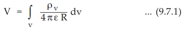
• For static electric fields, the electric scalar potential is given by,

• For static magnetic fields, the magnetic vector potential is given by,

• Let us now study the behaviour of these potentials when the fields are time varying.

• For time varying fields,

• As derived in earlier section, if we combine above relation with the expression of Faraday's law, we can write,

• It is clear from equations (9.7.3) and (9.7.4) that we can determine fields  provided that potentials V and Ā are known. It is necessary to find expressions for V and Ā, suitable for time varying fields.

• From the general field relations for time varying electric and magnetic fields,

• By taking divergence of equation (9.7.4) and using above two relations which are valid for time varying fields, we get

• It is important that complicated equations (9.7.5) and (9.7.7) are not sufficient enough to define Ā and V completely. These two equations demonstrate necessary but not the sufficient conditions. In general any vector field can be uniquely defined if its curl and divergence are known and the value of the field is known at any one point.

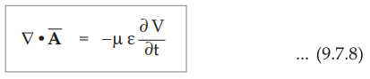
• The curl of Ā is already specified in the equation (9.7.3). Now we may choose the divergence of Ā from equation (9.7.7) as

• Equation (9.7.8) gives relationship between Ā and V. It is called Lorentz condition for potentials.

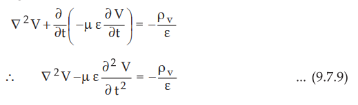
• Using the Lorentz condition in equation (9.7.5), we get,

• Similarly using Lorentz condition in equation (9.7.7), we get,

• Now equations (9.7.9) and (9.7.10) are very much symmetrical obtained from equations (9.7.5) and (9.7.7) by applying Lorentz condition for potentials. These are called wave equations.

• The solutions to the equation (9.7.9) and (9.7.10) are,

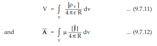
• The terms [ρv ] and [] in the equations (9.7.11) and (9.7.12) respectively, indicates that the time t in the expression ρ v (x, y, z, t) and  (x, y, z, t) is replaced by the retarded time denoted by t'. The retarded time is given by,

t' = t – R/v .... (9.7.13)

where          R = |  | i.e. Distance between the differential element of charge being considered and the point at which potential is to be measured.

• The velocity of wave propagation is denoted by v and it is defined as, ... (9.7.14)

• In free space, v = c ≅ 3 × 10⁸ m/s, which is the speed of light in vacuum.

• Thus the potentials V and Ā, represented by equations (9.7.11) and (9.7.12) are called retarded electric scalar potential and retarded magnetic vector potential respectively.

Review Question

1. Explain briefly about retarded, potential. What is the significance of it ?