Sampling Distributions

SAMPLING DISTRIBUTIONS

The probability distribution of a sample statistic is often called the sampling distribution of the statistic.

Alternatively we can consider all possible samples of size n that can be drawn from the population, and for each sample we compute the statistic. In this manner we obtain the distribution of the statistic, which is its sampling distribution.

The sample mean

Let X₁, X₂, X₃,...,X_n denote the independent, identically distributed, random variables for a random sample of size n.

Then the mean of the sample or sample mean is a random variable defined by

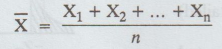
If x₁, x₂, ... X_n denote values obtained in a particular sample of size n, then the mean for that sample is denoted by

Example: If a sample of size 4 results in the sample values 7, 1, 6, 2 then the sample mean is

1. Sampling distribution of means

Let f(x) be the probability distribution of some given population from which we draw a sample of size n. Then it is natural to look for the probability distribution of the sample statistic   which is called the sampling distribution for the sample mean, or the sampling distributions of means.

Theorem: 1

The mean of the sampling distribution of means, denoted by , is given by  where µ is the mean of the population (or)

[A.U A/M 2018 R-08]

Prove that the expected value of the sample mean is the population mean.

Proof : Let the population be infinitely large and having a population mean of μ and a population variance of σ². If x is a random variable denoting the measurement of the characteristic, then

Expected value of x, E(x) = µ

Variance of x, Var (x) = σ²

The sample mean  is the sum of n random variables, viz., x₁, x₂, …. x_n, each being divided by n. Here, x₁, x₂, …. x_n are independent random variables from the infinitely large population.

Theorem: 2

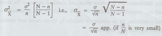
If a population is infinite and the sampling is random or if the population is finite and sampling is with replacement, then the variance of the sampling distribution of means denoted by  is given by

Where σ² is the variance of the population.

Theorem: 3

If the population is of size N, if sampling is without replacement, and if the sample size is n ≤ N, then

Theorem : 4

If the population from which samples are taken is normally distributed with mean μ and variance σ², then the sample mean is normally distributed

with mean μ and variance σ² / n

Theorem: 5

bas agisl

Testing of Hypothesis

slugog od 15.1

Suppose that the population from which samples are taken has a probability distribution with mean μ and variance σ² that is not necessarily a normal distribution, then the standardized variable associated with , given by

2. Sampling distribution of the proportion :

A simple sample of n items is drawn from the population. It is same as a series of n independent trials with the probability P of success.

The probabilities of 0, 1, 2, .., n successes are the terms in the binomial expansion of (p + q)^n.

Here mean = np and standard deviation = √npq.

Let us consider the proportion of successes, then

(a) Mean proportion of successes = np = P

(b) Standard deviation (standard error) of proportion of successes

= √npq / n  = √n/pq

(c) Precision of the proportion of success = 1/S.E. = √n/pq

3. Sampling distribution of differences and sums :

Suppose that we are given two populations. For each sample of size n₁ drawn from the first population, let us compute a statistic S₁. This yields a sampling distribution for S₁ whose mean and standard deviation we denote by μS₁ respectively. Similarly for each sample of size n2 drawn from the second population, let us compute a statistic S₂ whose mean and standard deviation are μS₂ and σS₂ respectively.

Taking all possible combinations of these samples for the two populations, we can obtain a distribution of the differences, S₁ – S₂, which is called the sampling distribution of differences of the statistics. The mean and standard deviation of this sampling distribution, denoted respectively by μS₁ - S₂ are given by

µ_S1 – S₂ = µ_S1 - µ_S2     σ_{S1 – S2} = σ²_{S1 – S}²₂ ….. (1)

provided that the samples chosen do not in any way depend on each other, i.e., the samples are independent (in other words, the random variables S₁ and S₂ are independent).

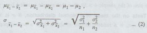
If, for example, S1 and S2 are the sample means from two populations, denoted by  respectively, then the sampling distribution of the differences of means is given for infinite populations with mean and standard deviation µ₁, µ₂ and µ₂ , σ₂ respectively by 

This result also holds for finite populations if sampling is with replacement. The standardized variable

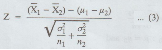
in that case is very nearly normally distributed if n1 and n2 are large (n1, n230). Similar results can be obtained for finite populations in which sampling is without replacement by using

and S₂ correspond to the proportions of successes P₁ and P₂ and equations (2) yield

Instead of taking differences of statistics, we sometimes are interested in the sum of statistics. In that case the sampling distribution of the sum of statistics S1 and S2 has mean and standard deviation given by

Assuming the samples are independent, results similar to (2) can then be obtained.

4. Sampling distribution of the variance :

We use a sample statistic called the sample variance to estimate the population variance. The sample variance is usually denoted by s².