Test Based on x2- Distribution

TEST BASED ON x²-DISTRIBUTION

a. x²-test for single variance

Let x₁, x₁,...,x₁ be a random sample from a normal population with variance σ². Set the null hypothesis' H₀ : σ² = σ²₀ Then the test statistic is

where s² is the variance of the sample.

Then  defined above follows a x²-distribution with n - 1 degrees

By comparing the calculated value of x² with the table value of x² for n-1 degrees of freedom at any required level of significance we may accept or reject the null hypothesis.

Note : If the sample size n is large (n > 30) then we can apply Fisher's approximation

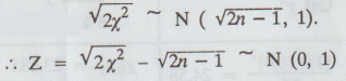
and we can apply normal test.

Example 1.4.a(1)

A random sample of size 25 from a population gives the sample standard deviation 8.5. Test the hypothesis that the population s.d is 10.

Solution :

Example 1.4.a.(2)

The s.d of the distribution of times taken by 15 workers for performing a job is 6.4 sec. Can it be taken as a sample from a population whose s.d is 5 sec ?

Solution :

Example 1.4.a(3)

It is believed that the precision (as measured by the variance) of an instrument is no more than 0.16. Write down the null and alternative hypothesis for testing this belief. Carry out the test at 1% level given 11 measurements of be in the same subject on the instrument. [A.U A/M 2017 R-13]

2.5, 2.3, 2.4, 2.3, 2.5, 2.7, 2.5, 2.6, 2.6, 2.7, 2.5

Solution :

Given: n = 11, σ² = 0.16

4. Conclusion :

Here Cal x² < table x²

i.e., 1.182 < 23.209

So, we accept H₀: σ² = 0.16

We conclude that the data are consistent with the hypothesis that the precision of the instrument is 0.16.

Example 1.4.a.(4)

Test the hypothesis that σ = 10, given that s = 15 for a random sample of size 50 from a normal population.

Solution: Given: σ = 10, s = 15, n = 50

6. Conclusion :

Since, |z| > 3, so we reject H₀, it is significant at all levels of significance. We conclude that σ ≠ 10

Example 1.4.a(5)

In the past the standard deviation of weights of certain 1135 gm packages filled by a machine was 7.1 gms. A random sample of 20 packages showed a standard deviation of 9.1 gms. Is the apparent increase in variability significant at 0.05 level of significance?

Solution: Given: n = 20, s = 9.1, σ = 7.1 ⇒ σ² =  50.41

1. H₀ σ² = 50.41

2. H₁ σ² ≠ 50.41

3.

4. Conclusion

Here, Cal x² > table x²

i.e., 32.855 > 30.144

So, we reject H₀ : σ² = 50.41

EXERCISES 1.4(a)______

1. A sample of 20 observations gave a standard deviation 3.72. Is this compatible with the hypothesis that the sample is from a normal population with variance 4.35.

2. A random sample of size 20 from a population gives the sample standard deviation of 6. Test the hypothesis that the population standard deviation is 9.

3. Given 11 measurements of an instrument as 2.5, 2.3, 2.4, 2.3, 2.5, 2.7, 2.6, 2.6, 2.7, 2.5. It is believed that the precision of that instrument as measured by the variance is 0.16. Test whether the data are consistent with the hypothesis (at 1% level of significance).

4. A sample of 12 values shows the s.d. to be 11. Does this agree with the hypothesis that the population s.d is 10, the population being normal ?

5. Weights in kgs of 10 students are given as 28, 40, 45, 53, 47, 43, 55, 48, 45, 49. Can we say that variance of the distribution of weights of all students from which the above sample of 10 students was drawn is equal to 20 kgs.