Testing of Hypothesis

UNIT – I

Chapter - 1

TESTING OF HYPOTHESIS

 

Introduction

Many problems in engineering require that we decide whether to accept or reject a statement about some parameter. The statement is called a hypothesis and the decision-making procedure about the hypothesis is called hypothesis testing. This is one of the most useful aspects of statistical inference, since many types of decision making problems, tests, or experiments in the engineering world can be formulated as hypothesis-testing problems. Furthermore, as we will see, there is a very close connection between hypothesis testing and confidence intervals. Statistical hypothesis testing and confidence interval estimation of parameters are the fundamental methods used in the data analysis stage of a comparative experiment.

Before giving the notion of sampling, we will first define population.

(a) Population

A population in statistics means a set of objects or mainly the set of numbers which are measurements or observations pertaining to the objects. The population is finite or infinite according to the number of elements of the set is finite or infinite.

(b) Sampling

A part selected from the population is called a sample. The process of selection of a sample is called sampling.

(c) Random sampling

A Random sampling is one in which each number of population has an equal chance of being included in it. There are NC_n different samples of size n that can be picked up from a population size N.

(d) Parameters and statistics

The statistical constants of the population, such as mean (µ), standard deviation (σ) are called parameters.

Parameters are denoted by Greek letters.

The mean x, standard deviation S of a sample are known as statistics. Statistics are denoted by Roman letters.

(e) Symbols for population and samples

(f) Aims of a sample

The population parameters are not known generally. Then, the sample characteristics are utilised to approximately determine or estimate the population. Thus, statistic is an estimate of the parameter. The estimate of mean and standard deviation of the population is a primary purpose of all scientific experimentation. The logic of the sampling theory is the logic of induction. In induction, we pass from a particular (sample) to general (population). This type of generalization here is known as statistical inference. The conclusion in the sampling studies are based not on certainties but on probabilities.

(g) Types of sampling

(1) Purposive sampling, (2) Random sampling, (3) Stratified sampling and (4) Systematic sampling.

(h) Sampling distribution

From a population, a number of samples are drawn of equal size n. Find out the me mean of each sample. The means of samples are not equal. The means with their respective frequencies are grouped. do algse 15llib On T The frequency distribution so formed is known as sampling distribution of the mean. Similarly, sampling distribution of standard deviation can be had.

(i) Standard error (S.E)

S.E is the standard deviation of the sampling distribution. For assessing the difference between the expected value and observed value, standard error is used.

Reciprocal of standard error is known as precision

If i is any statistic, for large samples Z = t – E (t) / S.E (t) is normaly distributed is normaly distributed with mean zero and variance unity.

i.e., Z = t – E (t) / S.E. (t) – N (0,1)

(j) Tests of significance

An important aspect of the sampling theory is to study the test of significance, which will enable us to decide, on the basis of the results of the samples, whether

(i) the deviation between the observed sample statistic and the hypothetical parameter value or

(ii) the deviation between two sample statics is significant or might be attributed due to chance or the fluctuations of the sampling.

If n is large, all the distributions like Binomial, Poisson, Chi-square, t distribution, F distribution can be approximated by a normal curve.

(k) Testing a hypothesis  [A.U CBT N/D 2011]

On the basis of sample information, we make certain decisions about the population. In taking such decisions, we make certain assumptions. These assumptions are known as statistical hypothesis. There hypothesis are tested.

Assuming the hypothesis is correct, we calculate the probability of getting the observed sample. If this probability is less than a certain assigned value, the hypothesis is to be accepted, otherwise rejected.

(l) Null hypothesis [H₀]

Null hypothesis is based on analysing the problem.

Null hypothesis is the hypothesis of no difference.

Thus, we shall presume that there is no significant difference between the observed value and expected value.

Then, we shall test whether, then this hypothesis is satisfied by the data or not.

If the hypothesis is not approved, then the difference is considered to be significant.

If the hypothesis is approved, then the difference would be attributed to sampling fluctuation.

Note: Null hypothesis is denoted by H₀.

(m) Alternative Hypothesis (H₁)

Any hypothesis which is complementary to the null hypothesis (H₀) is called an alternative hypothesis, denoted by H₁

Rule

(i) If we want to test the significance of the difference between a statistic and the parameter or between two sample statistics, then we set up the to null hypothesis that the difference is not significant.

This means that the difference is just due to fluctuations of sampling H₀: μ = x.

 (ii) If we want to test any statement about the population, then we set up the null hypothesis that it is true. For example, when we want to find, if the population mean has specified value uo, then we set up the null hypothesis H₀μ = μ0

(iii) Suppose, we want to test the null hypothesis that the population has a specified mean μo, that is,

H₀ : μ = µ₀, then the alternative hypothesis will be

(i) H₁ : μ ≠ µ₀ i.e., μ > µ₀  or μ < µ₀

(ii) H₁: μ > µ₀

(iii) H₁: μ < µ₀

H₁ in (i) is called a two-tailed alternative hypothesis

H₁ in (ii) is called a right-tailed alternative hypothesis

H₁ in (iii) is called a left-tailed alternative hypothesis

One has to set the alternative hypothesis clearly so that it will help us to decide to use a single - tailed (right or left) or two-tailed test.

(n) Critical region  [A.U Tvli. M/J 2011] [A.U N/D 2017 R-8]

A region, corresponding to a statistic t, in the sample space S which amounts to rejection of the null hypothesis Ho is called as critical region or region of rejection.

The region of the sample space S which amounts to the acceptance of Ho is called acceptance region.

(o) Critical value or significant value

The value of the test statistic which separates the critical region from the acceptance region is called the critical value or significant value.

(p) Level of significance [A.U. N/D 2013]

The probability that the value of the statistic lies in the critical region is called the level of significance.

In general, these levels are chosen as 0.01 or 0.05, called 1% level and 5% level of significance respectively.

(q) Errors  [A.U N/D 2011, A.U CBT A/M 2011] [A.U A/M 2015 R-8] [A.U M/J 2016 (R13)]

In sampling theory to draw valid inferences about the population parameter on the basis of the sample results, we decide to accept or to reject Ho after examining a sample from it. To av

Type I Error: If H₀ is rejected, while it should have been accepted.

Type II Error: If H₀ is accepted, while it should have been rejected.

(r) Large Sample Tests

Now we consider the following tests, under large sample test.

1. Test for a specified mean

2. Test for the equality of two means

3. Test for specified proportionatel

4. Test for equality of two proportions

(s) Test for a specified mean

A random sample of size n (n ≥ 30) is drawn from a population.

We want to test that the population mean has a specified value Mo

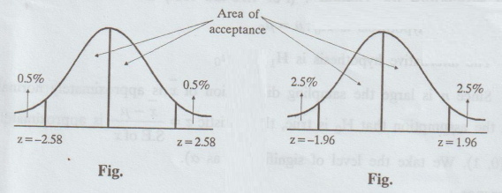
(t) Procedure for Testing (For two-tail test)

The null hypothesis is H₀ : μ = μ₀

The alternative hypothesis is H₁ : μ ≠ μ₀

Since n is large the sampling distribution of  is approximately normal.

(on the assumption that H₀ is true, the statistic z =  is approximately N (0, 1). We take the level of significance as ɑ).

Inference:

For a significance level a = 0.05 (5% level) if |z| < 1.96, H₀ is accepted at 5% level.

If |z| > 1.96, H₀ is rejected at 5% level

For ɑ = 0.01 (1% level of significance)

if |z|  < 2.58, H₀ is accepted at 1% level of significance.

if |z| > 2.58, H₀ is rejected at 1% level of significance.

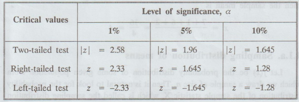
(u) Procedure for one-tailed test (left-tail)

(i) H₀ : μ ≥  μ₀

H₁: μ < μ₀ (left-tailed)

At ɑ : 0.05 the critical value

of |z |= 1.645

If z <-1.645, H₀ is rejected

If z > -1.645, H₀ is accepted

At ɑ = 0.01, the critical value of z is 2.33

(ii) One-tailed test (right-tailed)

If z < 1.645, H₀ is accepted.

z > 1.645, H₀ is rejected.

In all these cases, the test we apply, is called z-test.

(v) Table for critical values on using the normal probability

(w) Confidence limits

If a sample statistics lies in the interval

(µ - 1.96 σ, μ+ 1.96 σ), we call 95% confidence interval.

Similarly, Confidence limits as the area between μ - 2.58 σ and μ + 2.58 σ is 99%.

The numbers 1.96, 2.58 are called confidence co-efficients.