x2-test to test the goodness of fit

b. x²-test to test the goodness of fit.

A very powerful test for testing the significance of the discrepancy between theory and experiment was given by prof. Karl-Pearson in 1990 and is known as "Chi-square test of goodness of fit". It enables us to find if the deviation of the experiment from theory is just by chance or is it really due to the inadequacy of the theory to fit the observed data.

I. Chi-Square Test for Goodness of fit

x²-test of goodness of fit is a test to find if the deviation of the experiment from theory is just by chance or it is due to the inadequacy of the theory too fit the observed data.

By this test, we test whether differences between observed and expected frequencies are significant or not.

x² - test statistic of goodness of fit is defined by

x² = ∑  (O − E)² / E , where

O → Observed frequency swoo

E→ Expected frequency

II. Application or uses of x² -distribution

(1) To test the "goodness of fit".

(2) To test the "independence of attributes".

(3) To test if the hypothetical value of the population variance is o2.

(4) To test the homogeneity of independent estimates of the population variance.

(5) To test the homogeneity of independent estimates of the population correlation coefficient.

III. Conditions for the application of x²-test. [AU N/D 2011]

(1) The sample observations should be independent.

(2) Constraints on the cell frequencies, if any, must be linear

 [e.g., Σ Ο_i =  ΣΕ_i]

(3) N, the total frequency, should be atleast 50.

(4) No theoretical cell frequency should be less than 5.

 

IV. Independence of attributes

Note 1 In the case of

fitting a Binomial distribution, d.f = n - 1

fitting a Poisson distribution, d.f = n - 2

fitting a Normal distribution, d.f = n - 3

Note 2 If x² = 0, all observed and expected frequencies coincide

Note 3 For x²-distribution, mean = v, Variance = 2v

 

Example 1.4.b(1)

A company keeps records of accidents. During a recent safety review, a random sample of 60 accidents was selected and classified by the day of the week on which they occured.

Test whether there is any evidence that accidents are more likely on some days than others.

Solution:

The parameter of interest is to test whether there is any evidence that accidents are more likely on some days then others. So, we apply x² test.

1. H₀ : Accidents are equally likely to occur on any day of the week.

2. H₁ : Accidents are not equally likely to occur on the days of the week.

3. On the assumption H₀, the expected number of accidents on any day 60 / 5 = 12.

O → Observed frequency, E → Expected frequency

d.f = V = n − 1, Since ΣE (=ΣO) has been found using the sample data.

4. Conclusion:

Here, Cal x² < table x²

i.e., 4.499 < 9.488

So, we accept H₀

i.e., accidents may be regarded to occur uniformly over the week.

This means that the accidents are equally likely to occur on any day of the week.

 

Example 1.4.b(2)

The following data gives the number of aircraft accidents that occured during the various days of a week. Find whether the accidents are uniformly distributed over the week.

Solution :

The parameter of interest is to test the accidents are uniformly distributed. So, we apply x² test.

1. H₀ The accidents are uniformly distributed over the week.

2. H₁: The accidents are not uniformly distributed.

3. On the assumption of H_o, the expected number of accidents on any

day E = 84 / 7 = 12

O → Observed frequency, E→ Expected frequency

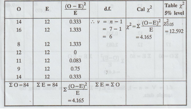
d.f = V = n 1, since ΣE (=ΣO) has been found using the sample data.

4. Conclusion:

Here, Cal x² < table x²

i.e., 4.165 < 12.592

So, we accept H₀

i.e., accidents are uniformly distributed over the week. stemsx

 

Example 1.4.b(3)

The table below gives the number of aircraft accidents that occurred during the various days of the week. Test whether the accidents are uniformly distributed over the week.

Sol. The parameter of interest is to test the accidents are uniformly distributed. So we apply x² test

1. H₀ : The accidents are uniformly distributed over the week.

2. H₁ : The accidents are not uniformly distributed

3. On the assumption of H₀, the expected number of accidents on any day = 90 / 6 = 15

O → Observed frequency, E→ Expected frequency

d.f = V = n − 1, since ΣE (= ΣO) has been found using the sample data.

4. Conclusion:

Here, Cal x² < table x²

i.e., 2.001 < 11.07

So, we accept H₀

This means that the accidents are uniformly distributed over the week.

 

Example 1.4.b(4)

In 120 throws of a single die, the following distribution of faces was observed.

Can you say that the die is biased

Solution: Given: n = 6

The variable of interest is to test if the die is biased. So we apply x² test.

1. H₀ The die is unbiased.

2. H₁ : The die is biased.

3. On the assumption H₀, the expected frequency (E) for each face

= 120 /  6 = 20

O → Observed frequency, E → Expected frequency

d.f = V = n − 1, since ΣE (=ΣO) has been found using the sample data.

4. Conclusion:

Here, Cal x² > table x²

i.e., 12.9 > 11.07

So, we reject H₀

Hence, the die can be regarded as biased.

 

Example 1.4.b(5)

A sample analysis of examination results of 500 students was made. It was found that 220 students have failed, 170 have secured a third class, 90 have secured a second class and the rest, a first class. So do these figures support the general belief that the above categories are in the ratio 4:3: 2:1 respectively?

Solution: Given: n = 4, 4 + 3 + 2 + 1 = 10

The variable of interest is the results in the four categories.

1. H₀ : The results in the four categories are in the ratio 4:3:2:1

2. H₁ The results in the four categories are not in the ratio 4:3:2:1

3. On the assumption Ho, the expected frequencies of the 4 classes are 3

4 / 10 × 500, 3 / 10 × 500, 2/ 10 × 500, 1 / 10 × 500

i.e., 200, 150, 100, 50

O → Observed frequency, E → Expected frequency visado 0

d.f= V = n 1, since Σ E (=Σ O) has been found using the sample data.

4. Conclusion :

Here, Cal x² > table x²

i.e., 23.667 > 7.815

So, we reject H₀ at 5% level of significance.

The results of the four categories are not in the ratio 4 : 3 : 2 : 1

 

Example 1.4.b(6)

A sample analysis of examination results of 1000 students were made and it was found that 260 failed, 110 first class, 420 second class and rest obtained third class. Do these data support the general examination result in the ratio 2 : 1 : 4: 3. [A.U N/D 2019 (R-17)]

Solution: Given: n = 4, 2 + 1 + 4 + 3 = 10

The variable of interest is the results in the four categories.

1. H₀ : The results in the four categories are in the ratio 2:1:4:3

2. H₁ The results in the four categories are not in the ratio 2:1:4:3

3. On the assumption H₀, the expected frequencies of the 4 classes are

2 / 10 × 1000, 1 / 10 × 1000, 4 / 10 × 1000, 3 / 10 × 1000 i.e.,  200, 100, 400, 300

O → Observed frequency, E → Expected frequency

d.f = V = n-1, since ΣE (=ΣO) has been found using the sample data.

4. Conclusion: ads ni sand soilingia to consbivo ai T ore

Here, Cal x² > table x²

i.e., 47 > 7.815

So, we reject H₀ at 5% level of significance.

The results of the four categories are not in the ratio 2:1:4:3.

 

Example 1.4.b.(7)

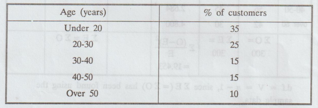
A company carries out regular market research to obtain information about the customers. It is particularly important to know the age distribution of the customers. In the recent years this has remained fairly constant and is shown in the following table.

A random sample of 300 customers selected during the latest market research investigation included the following numbers in each age group. Employ a Chi-square test to examine whether there is an evidence of significant change in the age distribution.

Solution :

The parameter of interest is to examine whether there is evidence of significant change in the age distribution.

1. H₀ : There is no evidence of significant change in the age distribution of customers.

2. H₁ : There is evidence of significant change in the age distribution of customers.

3. On the assumption H₀, the expected frequencies are

35 × 3, 25 × 3, 15 × 3, 15 × 3, 10 × 3

i.e., 105, 75, 45, 45, 30

O → Observed frequency, E→ Expected frequency attest

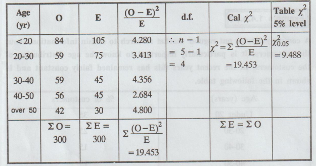
d.f = V = n − 1, since ΣE (= ΣO) has been found using the sample data.

4. Conclusion:

Here, Cal x² > table x²

i.e., 19.453 > 9.488

So, we reject H₀ at 5% level of significance

Hence there is evidence of significant change in the age distribution of customers.

 

Example 1.4.b (8)

Five coins are tossed 320 times. The number of heads observed is given below

Examine whether the coin is unbiased. Use 5% level of significance.

Solution: Here n = 6  [A.U A/M 2018 R-13]

1. H₀ : The coins are unbiased.

2. H₁: The coins are b

3. Probability of getting head p = 1/ 2

Probability of getting tail q = 1 / 2

Then the expected frequencies are

d.f v = n - 1, since ΣE (=ΣO) has been found using the sample data.

The value of p and q have not been found by using the sample data.

4. Conclusion:

Here Cal x² > table x²

i.e., 17.5 > 11.07

So, we reject H₀

Therefore the coins are biased.

 

Example 1.4.b(9)

4 coins were tossed 160 times and the following results were obtained:

Under the assumption that the coins are unbiased, find the expected frequencies of getting 0, 1, 2, 3, 4 heads and test the goodness of fit.

Solution: Here n = 5   [AU A/M 2011]

1. H₀ : The coins are unbiased

2. H₁: The coins are biased

3. Probability of getting head = p = 1 / 2

Probability of getting tail = q = 1 / 2

Then the expected frequencies are

d. f. = V = n − 1, since only ΣE (= ΣO) has been found using the sample data. The values of p and q have not been found by using the sample data.

4. Conclusion: Here, Cal x² > table x²

i.e., 12.73 > 9.488

So, we reject H₀

Therefore the coins are biased.

 

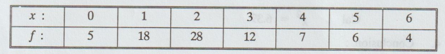
Example 1.4.b(10)

Fit a binomial distribution for the following data and also test the goodness of fit.

Solution :

1. H₀ : Binomial fit is satisfactory.

2. H₁ : Binomial fit is not satisfactory.

3. To find the binomial distribution N (q+p)ⁿ, which fits the given data we require p.

Converting E's into whole number such that ΣE = ΣO noiulono

Expected frequency in each class ≥ 10, Hence regroup.

ΣE (=ΣO) and p, q was found through its mean

The values of p and q have been found by using the sample data.

Hence d.f = v = n – k = n - 2

d.f = n - 2 = 4 - 2 = 2

Table x²0.05 = 5.99

Cal x² = 6.39

4. Conclusion :

Here Cal x² > table x²

i.e., 6.39 > 5.99

So, we reject H₀

Therefore the binomial fit is not satisfactory.simonid od ban of

 

Example 1.4.b(11)

A survey of 320 families with 5 children each revealed the following distribution:

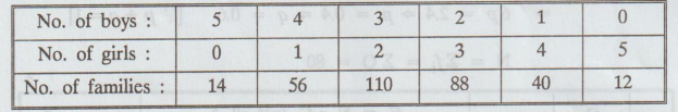
Is this result Consistent with the hypothesis that male and female births are equally probable ?

Solution :

1. H₀ : Male and Female births are equally probable gr

2. H₁: Male and Female births are not equally probable

3. On the assumption H₀, the expected frequencies are given by St the terms of N (q+p)ⁿ

d.f = v = n − 1, since ΣE (=Σ O) has been found using the sample

The values of p and q have not been found by using the sample data.

4. Conclusion:

Here,

Cal x² < table x²

i.e., 7.16 < 11.07

So, we accept H₀

i.e., make and female births are equally probable.

 

Example 1.4.b(12)

Twelve dice were thrown 4096 times and a throw of six was considered a success. The observed frequencies were as given below :

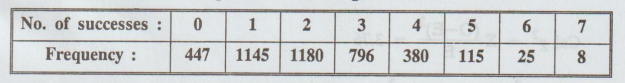
Test whether the dice were unbiased.

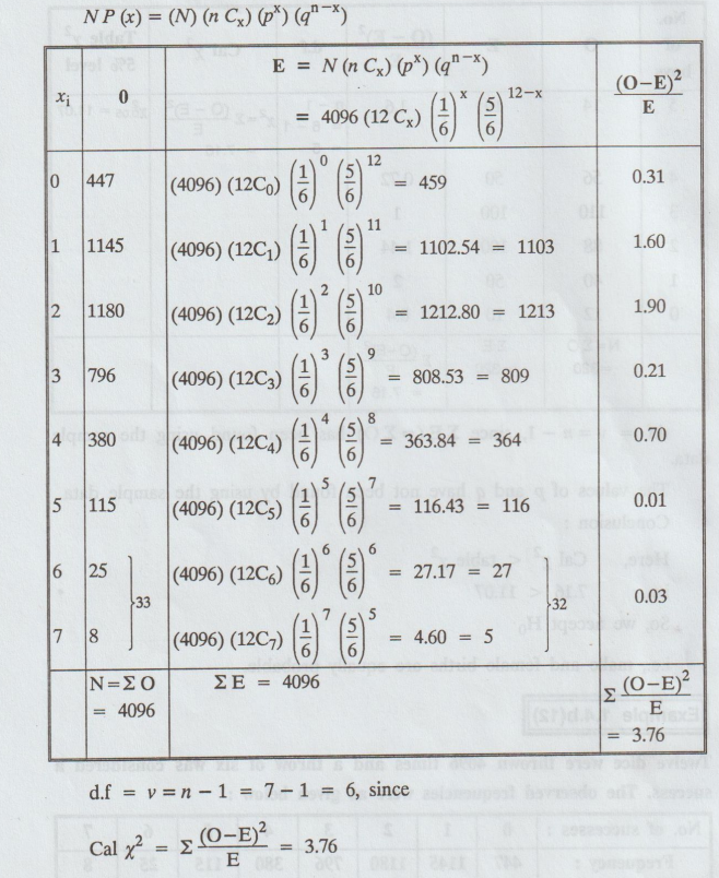
Solution: Given: n = 12

1. H₀ : All the dice were unbiased.

i.e., P (getting 6) = p = 1 / 6  q = 5 / 6   [': p + q = 1]

2. H₁ : All the dice were biased.

3. The expected frequencies are

Table x² = ∑ (O – E)² / E = 3.76

• The values of p and q have not been found by using the sample data.

• Converting E's into whole number such that ΣE = ΣO

• Expected frequency in each class ≥ 10, Hence regroup.

4. Conclusion:

Here, Cal x² < table x²

i.e., 3.76 < 12.59

So, we accept H₀

i.e., the dice were unbiased..

 

Example 1.4.b(13)

Fit a Poisson distribution for the following distribution and also test the goodness of fit.

Solution :

1. H₀ : Poisson fit is a good fit.

2. H₁ : Poisson fit is not a good fit.

• Converting E_i's into whole number such that Σ E = Σ O

• Expected frequency in each class 10, Hence regroup.

• ΣE (=ΣO) was found through its mean, Hence d.f = n - 2

4. Conclusion:

Cal x² < table x²

i.e., 1.09 < 5.99

So, we accept H₀, which assumes that the given distribution is nearly Poisson.

 

Example 1.4.b(14)

Fit a Poisson distribution to the given data and test the goodness of fit at 5 percent level of significance.

Solution :

1. H₀ : Poisson fit is a good fit.

2. H₁ : Poisson fit is not a good fit.

• Converting E's into whole number such that Σ E = Σ O.

• Expected frequency in each class ≥ 10. Hence regroup.

• ΣE (=ΣO) was found through its mean, Hence d.f = n - 2

4. Conclusion :

Cal x² > table x²

i.e., 41.04 > 5.991

So, we reject H₀. Hence we conclude that Poisson fit is not a good fit.

 

Example 1.4.b(15)

Theory predicts that the proportion of beans in four groups A, B, C, D should be 9:3:3: 1. In an experiment among 1600 beans, the numbers in the four groups were 882, 313, 287 and 118. Does the experiment support [A.U M/J 2012, M/J 2016]

the theory?

Solution :

1. H₀ : The experiment support the theory

2. H₁ : The experiment doesnot support the theory

3. On the assumption Ho, the expected frequencies are

4. Conclusion:

Here, Cal x² < table x²

i.e., 4.72 < 7.82

So, we accept H₀

Hence the experiment support the theory.

 

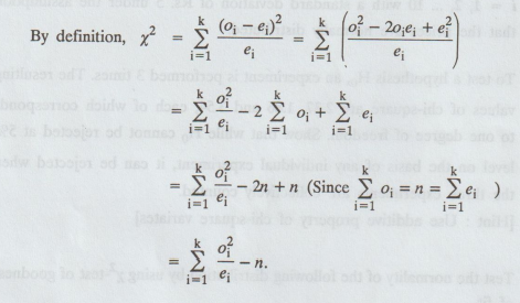
Example 1.4.b.(16)

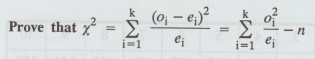
where there are k set of theoretical and observed values with the total frequencies n.

Solution :

 

EXERCISES 1.4(b)

1. In an experiment on pea-breeding, Mendal obtained the following frequencies of seeds: 315 round and yellow, 101 wrinkled and yellow; 108 round and green, 32 wrinkled and green. Total 556. Theory predicts that the frequencies should be in the proportion 9:3:3: 1 respectively. Set up proper hypothesis and test it at 10% level of significance.

Ans. x²  = 0.51. There seems to be good correspondence between theory and experiment.

2. Among 64 offsprings of a certain cross between guinea pigs, 34 were red, 10 were black and 20 were white. According to the genetic model these numbers should be in the ratio 9: 3: 4. Are the data consistent with the model at 5% level?

[You are given that the value of x² with the probability 0.05 being exceeded is 5.99 for 2. d.f. and 3.84 for 1 d.f.]

3. The following independent observations were made on the price of grain in 10 consecutive months :

Test the hypothesis that the expected price in the ith month is Rs. (100+3i), i = 1, 2, ... 10 with a standard deviation of Rs. 5 under the assumption that the prices are normally distributed. noitinilab ya

4. To test a hypothesis Ho, an experiment is performed 3 times. The resulting values of chi-square are 2.37, 1.86 and 3.54, each of which corresponds to one degree of freedom. Show that while Ho cannot be rejected at 5% level on the basis of any individual experiment, it can be rejected when the three experiments are collectively counted.

[Hint: Use additive property of chi-square variates]

5. Test the normality of the following distribution by using x2-test of goodness of fit.

6. Fit a normal distribution to the following data and test the goodness of fit.

7. The following data represents the monthly sales (in Rs.) of a certain retail stores in a leap year. Examine if there is any seasonality in the Just sales.

6100, 5600, 6350, 6050, 6250, 6200, 6300, 6250, 5800, 6000, 6150 and 6150