Lagrange's Interpolation

LAGRANGE'S INTERPOLATION

The Lagrangian polynomial method is a very straight forward approach. The method perhaps is the simplest way to exhibit the existence of a polynomial for interpolation with uneven spaced data. Data, where the x-values are not equi-spaced often occur as the result of experimental observations or when historical datas are examined.

Suppose, we have a table of data with four pairs of x and f (x) values. With x; indexed by variable 'i':

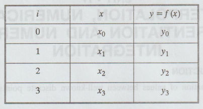
Here, we do not assume uniform spacing between the x-values, nor we need the x-values arranged in a particular order. All the x-values must be distinct, however, through these four data pairs, we can pass a cubic. The Lagrangian form for this is

The arithmetic in this method is tedious, although hand calculators are convenient for this type of computation. Writing a computer program that implements the method is not hard to do. Both MATLAB and Mathematica can get interpolating polynomials of any degree. An interpolating polynomial, although passing through the points used in its construction does not, in general, give exactly correct values when used for interpolation. The reason is that the underlying relationship is often not a polynomial of the same degree. We are interested in the error of interpolation.

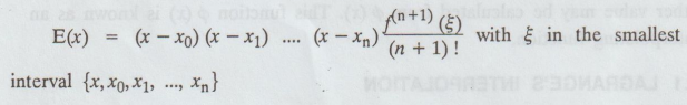
The expression for error is interesting but is not always extremely useful. We can conclude, however, that if the function is "smooth", a low-degree polynomial should work satisfactory. On the otherhand, a "rough" function can be expressed to have larger errors, when interpolated.

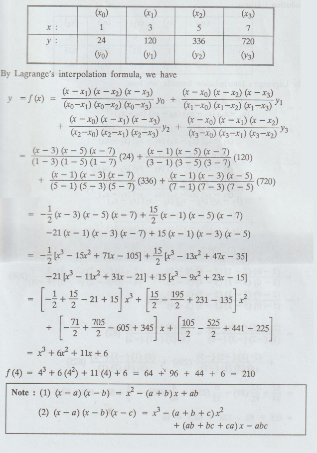
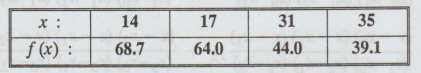
1. Find the polynomial f (x) by using Lagrange's formula and hence find f(3) for

Solution :

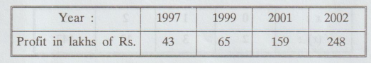
2. Using Lagrange's interpolation, calculate the profit in the year 2000 from the following data:

[A.U. April/May 2004, A.U M/J 2012]

Solution: Given:

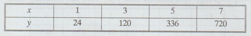
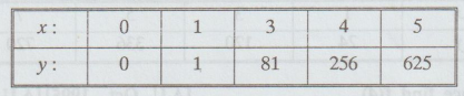
3. Find the third degree polynomial f(x) satisfying the following data:

Solution :

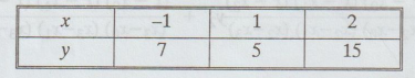
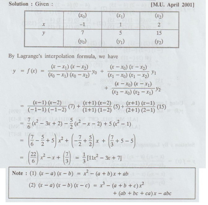
4. Using Lagrange interpolation find y (2) from the following data.

Solution: Given:

5. Using Lagrange's interpolation formula, find f(4) given that f(0) 2, f(1) = 3, f(2) = 12, f(15) = 3587

Solution: Given

6. Using Lagrange's interpolation formula, find y(10) given that  y(5) = 12, y(6) = 13, y(9) = 14, y(11) = 16.

[MU.April, 1999]

[A.U M/J 2012, CBT N/D 2011] [A.U N/D 2019 R-13] [A.U N/D 2020 R-17 N/M] [A.U A/M 2021 R-17 NM] [A.U N/D 2021 R-17]

Solution:

7. Using Lagrange’s fprmula, fit a polynomial to the data

Solution : Given

8. The mode of a certain frequency curve y = f(x) is very nearer to x = 9 and the values of the frequency density f(x) for x = 8.9, 9, 9.3 are 0.30, 0.35 and 0.25 respectively. Calculate the approximate value of the mode.

Solution: Given:

9. Using Lagrange's formula, prove y₁ = y₃ - 0.3 (y₅y_-3) + 0.2 (y_-3 + y_-5) nearly.

Solution:

Here, y_-5, y_-3, y₃, y₅ are the terms in the given expression. So, we have the table

10. Find the parabola is of the form y = ax² + bx + c passing through the points (0, 0), (1, 1) and (2, 20).

Solution: By Lagrange's interpolation formula, we have

11. Find the Lagrangian interpolating polynomial for the following data:

12. Use Lagrange's method to find log₁₀ 656, given that log₁₀ 654 = 2.8156, log₁₀ 658 = 2.8182, log₁₀ 659 = 2.8189 and log₁₀ 661 = 2.8202

Solution: Given: [A.U N/D 2012]

13. Use Lagrange's formula to find the value of y at x = 6 from the following data: [A.U. N/D 2013]

14. Given the values

Find f(27) by using Lagrange's interpolation formula.

[A.U. N/D 2006] [A.U. M/J 2006] [A.U A/M 2019 R-17]

Solution:

Given:

15. Find the expression of f(x) using Lagrange's formula for the following data :